| neck (cm) | waist (cm) | height (m) | weight (kg) | |
|---|---|---|---|---|
| count | 11.00000 | 11.000000 | 11.000000 | 11.000000 |
| mean | 33.90000 | 75.663636 | 48.140000 | 60.227273 |
| std | 8.20317 | 23.492010 | 79.691223 | 12.098272 |
| min | 13.50000 | 27.000000 | 1.580000 | 49.000000 |
| 25% | 32.00000 | 66.500000 | 1.650000 | 49.500000 |
| 50% | 36.00000 | 73.000000 | 1.740000 | 58.000000 |
| 75% | 38.60000 | 81.000000 | 80.910000 | 71.000000 |
| max | 44.70000 | 115.300000 | 180.000000 | 83.000000 |
Logistic Regression
INF-604: Data Analysis
![]()
Motivation
- Not all problems require us to predict
numbers! - For example:
- Is tomorrow raining or not?
- Can a certain individual pay back the loan on-time this month?
- May a certain individual have a certain type of disease?…
- The outcomes of these problems are just
yesorno(Not number).
Such problems are called
Classification problems.
Motivation
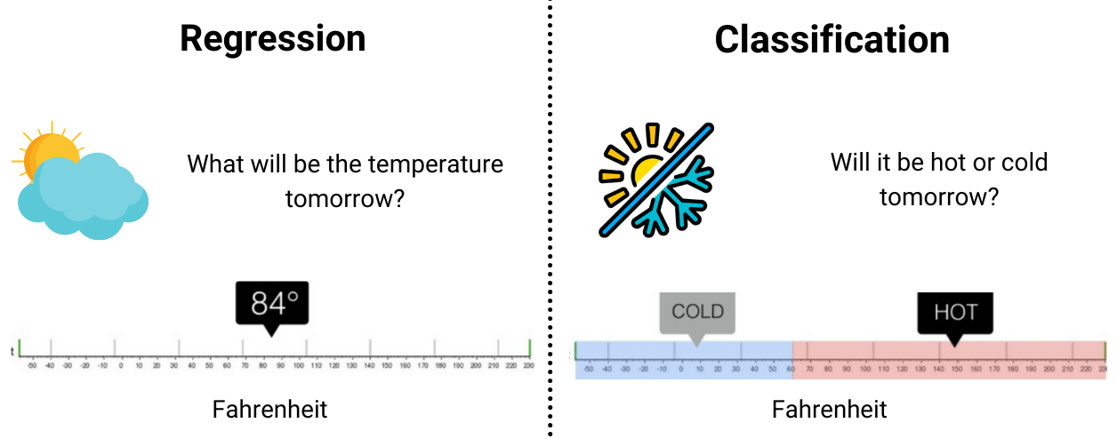
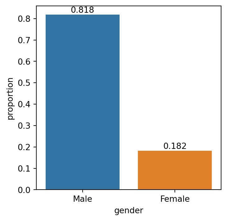
Linear Regressionaims at predictingquantitativetarget (number). Such a task is called Regression problem.Logistic Regressionaims at predictingcategoricaltarget (class/type). It’s a Classification model.- Consider a survey available here: Data Collection.
- What’s wrong with this data?
Binary Logistic Regression
Summary
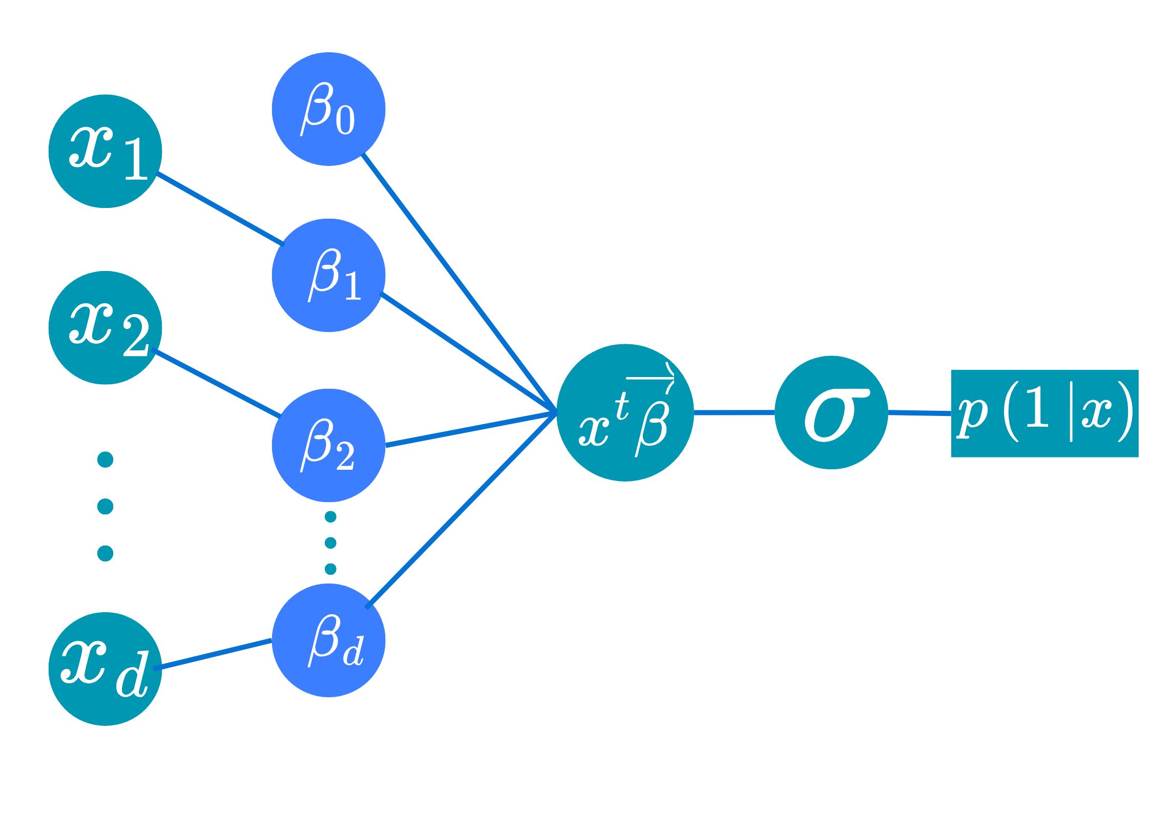
Logistic Regression Model
- Main model: \(p(1|\text{x})=1/(1+e^{-\color{green}{z}})=1/(1+e^{-(\color{blue}{\beta_0}+\text{x}^T\color{blue}{\vec{\beta}})})\).
- Interpretation:
- Boundary decision is
Lineardefined by the coefficients \(\color{blue}{\beta_0}\) and \(\color{blue}{\vec{\beta}}\). - Probability of being in each class depends on the relative distance of that point to the boundary.
- Works well when classes are linearly separable.
- Boundary decision is
- Interpretation:
- Objective: buliding a Logistic Regression model is equivalent to searching for parameters \(\color{blue}{\beta_0}\) and \(\color{blue}{\vec{\beta}}\) that minimizes the Cross-entropy.
- The loss cannot be minimized analytically but can be minimized numerically.
Logistic Regression
Application on Auto-MPG
- For our
Auto-MPGdataset, we aim at predictingoriginusing some characteristics of the cars. - Build intuition through visualization:
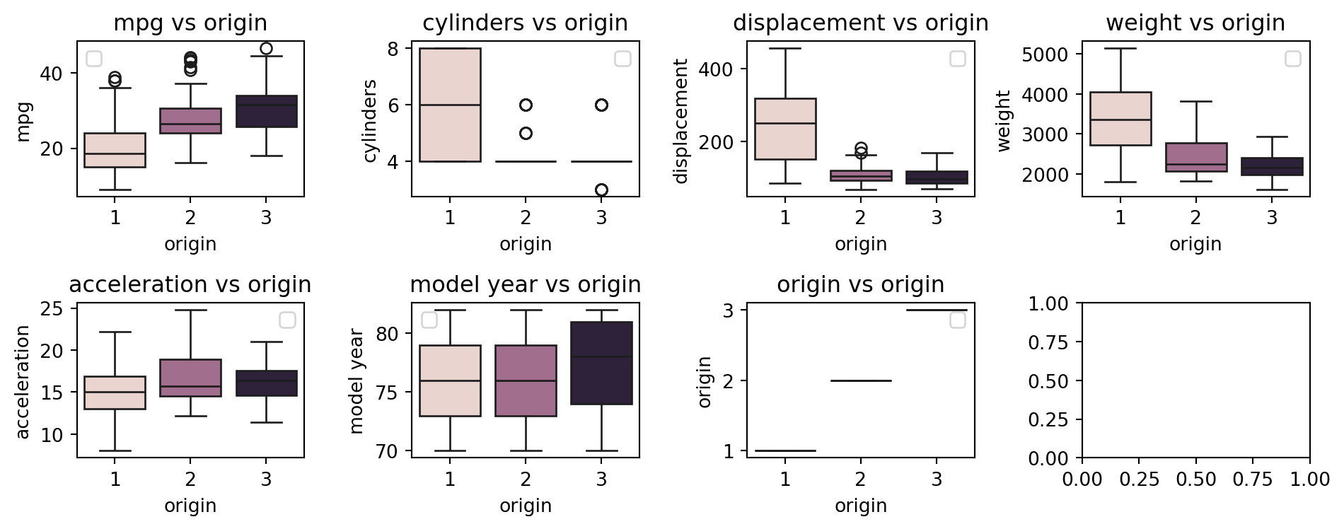
![]()