Advanced Machine Learning

     

Lecturer: Dr. HAS Sothea

Code: AMSI61AML

3. Logistic Regression & Regularization

Binary Logistic Regression

• Objective: classify whether \(y=0\) or \(1\) using its input \(\text{x}\in\mathbb{R}^d\).

• Classifying \(\Leftrightarrow\) identifying the decision boundary.

• A good decision boundary should separates classes well.

• Normally:

  • Far from it = more certain.
  • Close to it = less certain.

---

• Assumption: The decision boundary is linear.

x1	x2	y
-0.752759	2.704286	1
1.935603	-0.838856	0

import plotly.express as px
import plotly.graph_objects as go
fig = px.scatter(
    data_toy1, x="x1", y="x2", 
    color="y")

# Lines
line_coefs = np.array(
    [[1, 1, -2], [-1, 0.3, 0.5], [-0.5, 0.3, -1], [0.1, -1, 1]])
frames = []
x_line = np.array([np.min(x1[:,1]), np.max(x1[:,1])])
y_range = np.array([np.min(x1[:,2]), np.max(x1[:,2])])
id_small = np.argsort(np.abs(x1[:,1]) + np.abs(x1[:,2]))[5]
point_far = np.array([x_line[0], y_range[1]])
point_near = np.array([x1[id_small,1],x1[id_small,2]])

for i, coef in enumerate(line_coefs):
    y_line = (-coef[0] - coef[1] * x_line) / coef[2]
    a, b = -coef[1]/coef[2], -coef[0]/coef[2]
    point_proj_far = np.array([(point_far[0]+a*point_far[1]-a*b)/(a**2+1), a*(point_far[0]+a*point_far[1]-a*b)/(a**2+1)+b])
    point_proj_near = np.array([(point_near[0]+a*point_near[1]-a*b)/(a**2+1), a*(point_near[0]+a*point_near[1]-a*b)/(a**2+1)+b])
    p1 = np.row_stack([point_far, point_proj_far])
    p2 = np.row_stack([point_near, point_proj_near])
    frames.append(go.Frame(
        data=[fig.data[0],
              fig.data[1],
              go.Scatter(
                x=p1[:,0],
                y=p1[:,1],
                name="Far from boundary",
                line=dict(dash="dash"),
                visible="legendonly"
              ),
              go.Scatter(
                x=p2[:,0],
                y=p2[:,1],
                name="Close to boundary",
                line=dict(dash="dash"),
                visible="legendonly"
              ),
              go.Scatter(
                x=x_line, y=y_line, mode='lines',
                line=dict(width=3, color="black"), 
                name=f'Line: {i+1}')],
        name=f'{i+1}'))

y_line = (-line_coefs[0,0] - line_coefs[0,1] * x_line) / line_coefs[0,2]
a, b = -line_coefs[0,0]/line_coefs[0,2], - line_coefs[0,1]/line_coefs[0,2]
point_proj_far = np.array([(point_far[0]+a*point_far[1]-a*b)/(a**2+1), a*(point_far[0]+a*point_far[1]-a*b)/(a**2+1)+b])
point_proj_near = np.array([(point_near[0]+a*point_near[1]-a*b)/(a**2+1), a*(point_near[0]+a*point_near[1]-a*b)/(a**2+1)+b])
p1 = np.row_stack([point_far, point_proj_far])
p2 = np.row_stack([point_near, point_proj_near])
fig1 = go.Figure(
    data=[
        fig.data[0],
        fig.data[1],
        go.Scatter(
            x=p1[:,0],
            y=p1[:,1],
            name="Far from boundary",
            line=dict(dash="dash"),
            visible="legendonly"
            ),
        go.Scatter(
            x=p2[:,0],
            y=p2[:,1],
            name="Close to boundary",
            line=dict(dash="dash"),
            visible="legendonly"
        ),
        go.Scatter(
            x=x_line, y=y_line, mode='lines',
            line=dict(width=3, color="black"), 
            name=f'Line: 1')
    ],
    layout=go.Layout(
        title="1st simulated data & boundary lines",
        xaxis=dict(title="x1", range=[-3.4, 3.4]),
        yaxis=dict(title="x2", range=[-3.4, 3.4]),
        updatemenus=[{
            "buttons": [
                {
                    "args": [None, {"frame": {"duration": 1000, "redraw": True}, "fromcurrent": True, "mode": "immediate"}],
                    "label": "Play",
                    "method": "animate"
                },
                {
                    "args": [[None], {"frame": {"duration": 0, "redraw": False}, "mode": "immediate"}],
                    "label": "Stop",
                    "method": "animate"
                }
            ],
            "type": "buttons",
            "showactive": False,
            "x": -0.1,
            "y": 1.25,
            "pad": {"r": 10, "t": 50}
        }],
        sliders=[{
            "active": 0,
            "currentvalue": {"prefix": "Line: "},
            "pad": {"t": 50},
            "steps": [{"label": f"{i}",
                       "method": "animate",
                       "args": [[f'{i}'], {"frame": {"duration": 1000, "redraw": True}, "mode": "immediate", 
                       "transition": {"duration": 10}}]}
                      for i in range(1,5)]
        }]
    ),
    frames=frames
)

fig1.update_layout(height=370, width=500)

fig1.show()

Binary Logistic Regression

Model intuition

• If \((P):\beta_0+\sum_{j=1}^d\beta_jx_j=0\) is a boundary (hyperplane) with some orthogonal vector \(\vec{\beta}\in\mathbb{R}^d\), then for any input \(\text{x}_0\in\mathbb{R}^d:\) \[\color{green}{z_0}=\color{green}{\beta_0+\text{x}_0^T\vec{\beta}}\ \text{is the relative distance from }\text{x}_0\to (P).\]

• That’s to say that
  • \(\color{green}{z_0}>0\Leftrightarrow \text{x}_0\) is above the boundary \((P)\).
  • \(|\color{green}{z_0}|\) is large \(\Leftrightarrow\) \(\text{x}_0\) is far from \((P)\).

• \((P)\) is a good boundary:
  • \(|\color{green}{z_0}|\) large \(\Rightarrow\) “certain about its class”.
  • \(|\color{green}{z_0}|\) small \(\Rightarrow\) “less certain about its class”.

Binary Logistic Regression

Model intuition

• \((P)\) is a good boundary:
  • \(|\color{green}{z_0}|\) large \(\Rightarrow\) “certain about its class”.
  • \(|\color{green}{z_0}|\) small \(\Rightarrow\) “less certain about its class”.
• Sigmoid function, \(\sigma:\mathbb{R}\to (0,1)\)

\[\color{green}{z}\mapsto\sigma(\color{green}{z})=\frac{1}{1+\exp(-\color{green}{z})}.\]

Key ideas

• \(\color{green}{z_0}=\color{green}{\beta_0+\text{x}_0^T\vec{\beta}}\) is the relative distance of \(\text{x}_0\) w.r.t \((P)\).
• Sigmoid can converts this relative distance into probability.

Binary Logistic Regression

Model

• For any parameters \(\beta_0\in\mathbb{R},\vec{\beta}=(\beta_1,\dots, \beta_d)\in\mathbb{R}^d\), we assume for any input data \(\text{x}\in\mathbb{R}^d\) that the probability that \(\text{x}\) belongs to class \(1\) is given by

\[\begin{align*} \mathbb{P}(Y=1|X=\text{x})=\sigma(\beta_0+\text{x}^T\vec{\beta})=\frac{1}{1+\exp(-\beta_0-\text{x}^T\vec{\beta})}:=p(1|\text{x})=1-p(0|\text{x}). \end{align*}\]

• Interpretation:
  • \(\text{x}\) has relative distance \(z=\beta_0+\text{x}^T\vec{\beta}\) to the boundary defined by \(\beta_0\in\mathbb{R}\) and \(\vec{\beta}\in\mathbb{R}^d\).
  • This relative distance is converted to probability using sigmoid function: \(\sigma(z)\).
  • If \(z>>0\), then \(\text{x}\) is far above the boundary, and it is highly likely to be in class \(1\).
  • If \(z<<0\), then \(\text{x}\) is far below the boundary, and it is highly likely to be in class \(0\).
  • If \(z\approx 0\), \(\text{x}\) is close to the boundary, and its class is uncertain!
• The relative distance is known as log-odd:\[\text{Logit}(p(1|\text{x}_i))=\log\Big(\frac{p(1|\text{x})}{p(0|\text{x})}\Big)=\beta_0+\sum_{j=1}\beta_jx_{ij}.\]

Binary Logistic Regression

Example: 1st Simulated Data

• If \((\beta_0,\beta_1,\beta_2)=(1, 1, -2)\), compute \(p(1|\text{x})\) of the following data:

x1	x2	y
2.489186	-0.779048	0
-2.572868	-1.086146	1
2.767143	2.432104	0

• Compute relative distance \(z_i=\beta_0+\text{x}_i^T\vec{\beta}\), then \(p(1|\text{x}_i)\) \[\begin{align*}z_1&=1+1(2.489186)-2(-0.779048)\\ &=5.047282>0\\ \Rightarrow p(1|\text{x}_1)&=\sigma(z_1)=1/(1+e^{-5.047282})=\color{blue}{0.9936}.\\ \\ z_2&=1+1(-2.572868)-2(-1.086146)\\ &=0.599424>0\\ \Rightarrow p(1|\text{x}_2)&=\sigma(z_2)=1/(1+e^{-0.599424})=\color{blue}{0.6455}.\\ \\ z_2&=1+1(2.767143)-2(2.432104)\\ &=-1.097065 < 0\\ \Rightarrow p(1|\text{x}_3)&=\sigma(z_3)=1/(1+e^{-(-1.097065)})=\color{red}{0.2503}.\end{align*}\]

• Interpretation: \(\text{x}_1,\text{x}_2\) are located above the line \((P):1+x_1-2x_2\) and are predicted to be in class \(\color{blue}{1}\). On the other hand, \(\text{x}_3\) is located below the line and is predicted to be in class \(\color{red}{0}\).

• Next, we shall discuss how to define a criterion to obtain the optimal parameters \(\color{green}{\widehat{\beta_0}}\) and \(\color{green}{\widehat{\vec{\beta}}}\).

Binary Logistic Regression

Conditional likelihood

• Data: \({\cal D}=\{(\text{x}_1,y_1),...,(\text{x}_n,y_n)\}\subset\mathbb{R}^d\times \{0,1\}\).

• Objective: search for \(\beta_0\in\mathbb{R},\vec{\beta}\in\mathbb{R}^d\) such that the model is best aligned with the data \({\cal D}\): \[p(y_i|\text{x}_i)\text{ is large for all }i\in\{1,\dots,n\}.\]

• Conditional Likelihood Function: If the data are iid, one has \[\begin{align*}{L}(\beta_0,\vec{\beta})&=\mathbb{P}(Y_1=y_1,\dots,Y_n=y_n|X_1=\text{x}_1,\dots,X_n=\text{x}_n)\\ &=\prod_{i=1}^np(y_i|\text{x}_i)\\ &=\prod_{i=1}^n\Big[p(1|\text{x}_i)\Big]^{y_i}\Big[p(0|\text{x}_i)\Big]^{1-y_i}\\ &=\prod_{i=1}^n\Big[\sigma(\beta_0+\text{x}_i^T\vec{\beta})\Big]^{y_i}\Big[(1-\sigma(\beta_0+\text{x}_i^T\vec{\beta}))\Big]^{1-y_i}. \end{align*}\]

Binary Logistic Regression

Log Loss/Logistic Loss/Cross-entropy

• Log-Conditional Likelihood function: recall that \(p(1|\text{x}_i)=\sigma(\beta_0+\text{x}_i^T\vec{\beta})\) then \[\begin{align*}\log[L(\beta_0,\vec{\beta})]&=\sum_{i=1}^n\Big[y_i\log[p(1|\text{x}_i)]+(1-y_i)\log[p(0|\text{x}_i)]\Big].\qquad(1) \end{align*}\]

• Log-loss or logistic loss or Cross-entropy: \[\color{red}{{\cal L}(\beta_0,\vec{\beta})=-\log[L(\beta_0,\vec{\beta})]}.\]
• Objective: searching for \(\color{green}{\widehat{\beta}_0}\in\mathbb{R}\),\(\color{green}{\widehat{\vec{\beta}}}\in\mathbb{R}^d\) that minimizes \(\color{red}{{\cal L}(\beta_0,\vec{\beta})}\), i.e., \[{\cal L}(\color{green}{\widehat{\beta}_0,\widehat{\vec{\beta}}})=\inf_{\beta_0\in\mathbb{R},\vec{\beta}\in\mathbb{R}^d}\color{red}{{\cal L}(\beta_0,\vec{\beta})}.\]
• Ex: The 1st simulated data 👉

Binary Logistic Regression

Log Loss/Logistic Loss/Cross-entropy

• Log-Conditional Likelihood function: recall that \(p(1|\text{x}_i)=\sigma(\beta_0+\text{x}_i^T\vec{\beta})\) then \[\begin{align*}\log[L(\beta_0,\vec{\beta})]&=\sum_{i=1}^n\Big[y_i\log[p(1|\text{x}_i)]+(1-y_i)\log[p(0|\text{x}_i)]\Big]. \end{align*} \qquad(1)\]

• Log-loss or logistic loss or Cross-entropy: \[\color{red}{{\cal L}(\beta_0,\vec{\beta})=-\log[L(\beta_0,\vec{\beta})]}.\]
• Objective: searching for \(\color{green}{\widehat{\beta}_0}\in\mathbb{R}\),\(\color{green}{\widehat{\vec{\beta}}}\in\mathbb{R}^d\) that minimizes \(\color{red}{{\cal L}(\beta_0,\vec{\beta})}\), i.e., \[{\cal L}(\color{green}{\widehat{\beta}_0,\widehat{\vec{\beta}}})=\inf_{\beta_0\in\mathbb{R},\vec{\beta}\in\mathbb{R}^d}\color{red}{{\cal L}(\beta_0,\vec{\beta})}.\]
• Ex: The 1st simulated data 👉

def log_loss(beta1, beta2, X, y, beta0 = 0.1):
    beta_ = np.array([beta0, beta1, beta2])
    sig = sigmoid(X @ beta_)
    loss = np.mean(y*np.log(sig) + (1-y)*np.log(1-sig))
    return -loss

beta1 = np.linspace(-7,2,25)
beta2 = np.linspace(-2,7,30)
losses = np.array([[log_loss(b1, b2, X=x1, y=y_) for b1 in beta1] for b2 in beta2])
bright_blue1 = [[0, '#235b63'], [1, '#45e696']]
fig = go.Figure(go.Surface(
    x=beta1, y=beta2, z=losses, name="Loss function",
    colorscale=bright_blue1,
    hovertemplate='beta1: %{x}<br>' + 
                  'beta2: %{y}<br>' +
                  'Loss: %{z}<extra></extra>'))
fig.update_layout(
                scene = dict(
                xaxis_title= 'beta1',
                yaxis_title= 'beta2',
                zaxis_title='Loss'),
                width=450, height=300, title="Loss function of the 1st dataset")
fig.show()

Binary Logistic Regression

Properties of The Loss

• Log loss \({\cal L}:\mathbb{R}^{d+1}\to \mathbb{R}\) is convex [See: D. Jurafsky and J. H. Martin (2023)].
• Consequence: There exists a unique \((\color{green}{\widehat{\beta}_0,\widehat{\vec{\beta}}})\) that minimizes the loss \({\cal L}\), i.e.,

\[(\color{green}{\widehat{\beta}_0,\widehat{\vec{\beta}}})=\arg\min_{\beta_0\in\mathbb{R},\vec{\beta}\in\mathbb{R}^d}\color{red}{{\cal L}(\beta_0,\vec{\beta})}.\]

• 😭 Unfortunately, such minimizer values \((\color{green}{\widehat{\beta}_0,\widehat{\vec{\beta}}})\) cannot be analytically computed.

• 😊 Fortunately, it can be numerically approximated!

Binary Logistic Regression

Properties of The Loss (Continous)

• If \(P=(p_1,\dots,p_d)\) and \(Q=(q_1,\dots,q_d)\) are two probability vectors, then Kullback–Leibler (KL) divergence between \(P\) and \(Q\) is defined by \[\color{blue}{\text{KL}(P\|Q)}=\sum_{j=1}^dp_j\log\Big(\frac{p_j}{q_j}\Big)\]
  • It measures disimilarity between \(P\) and \(Q\).
  • Ex: \(P_1=(0.6, 0.3, 0.1),P_2=(0.5, 0.2, 0.3)\) and \(Q=(0.3, 0.4, 0.3)\)
    • \(\text{KL}(P_1\|Q)=\) 0.21972,
    • \(\text{KL}(P_2\|Q)=\) 0.11678 (suggesting that \(P_2\) is more similar to \(Q\) than \(P_1\)).
  • \(\text{KL}(P\|Q)\geq 0\) for any probability vectors \(P,Q\).
  • \(\text{KL}(P\|Q)= 0\Leftrightarrow P=Q\).
  • Note that, in general: \(\text{KL}(P\|Q)\neq \text{KL}(Q\|P)\).
• For any probab. vectors \(P\) and \(Q\): \(\color{red}{\text{CEn}(P,Q)}=-\sum_{j=1}^dp_j\log(q_j)\geq \color{blue}{\text{KL}(P\|Q)}, (Q:\text{ model})\).

Binary Logistic Regression

Summary

Logistic Regression Model

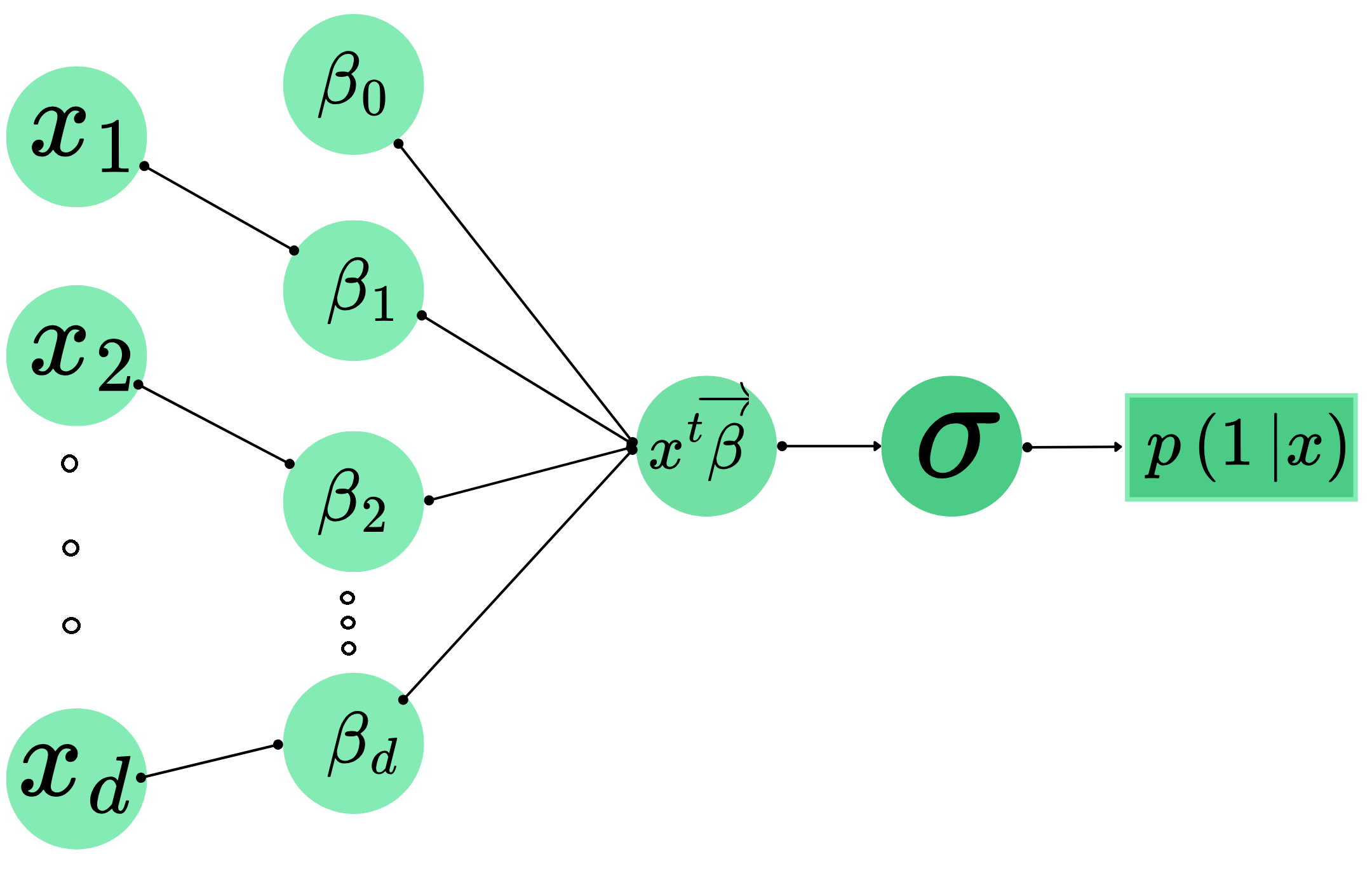
• Main assumption: \(p(1|\text{x})=1/(1+e^{-\color{green}{z}})=1/(1+e^{-\color{green}{(\beta_0+\text{x}^T\vec{\beta})}})\).
  • Interpretation:
    • Boundary decision is Linear (hyperplane) defined by \(\beta_0\) and \(\vec{\beta}\).
    • Probability of being in each class depends on the relative distance of that point to the boundary.
    • Works well when classes are linearly separable.

• Objective: buliding a Logistic Regression model is equivalent to searching for parameters \(\beta_0\) and \(\vec{\beta}\) that minimizes the Log Loss function (Equation 1).
• The loss cannot be minimized analytically but can be minimized numerically.

Binary Logistic Regression

Polynomial Features

• Linear boundary assumption might be too weak in real situation.
• Polynomial features: \(X_1,\dots,X_d\to X_i^kX_j^{p-k}, k=0,1,\dots,p\).

• Original data:

	x1	x2
0	-0.752759	2.704286
1	1.391964	0.591951
2	-2.063888	-2.064033

• Poly. features:

	x1	x2	x1^2	x1 x2	x2^2
0	-0.752759	2.704286	0.566647	-2.035676	7.313162
1	1.391964	0.591951	1.937563	0.823974	0.350406
2	-2.063888	-2.064033	4.259634	4.259933	4.260232

Binary Logistic Regression

Polynomial Features

• Linear boundary assumption might be too weak in real situation.
• Polynomial features: \(X_1,\dots,X_d\to X_i^kX_j^{p-k}, k=0,1,\dots,p\).

• Offer more flexible boundaries.
• May be more suitable in complex problems.
• Higher risk of overfitting!!!
• Overfitting: happens when a model learns the training data too well, capturing noise and fluctuations rather than the underlying pattern.

Binary Logistic Regression

Gradient

Gradient

• If \(L:\mathbb{R}^d\to\mathbb{R}, y=L(x_1,...,x_d)\) be a real-valued function of \(d\) real variables. For any point \(a\in\mathbb{R}^d\), the gradient of \(L\) at point \(a\) is a \(d\)-dimensional vector defined by \[\nabla L(a)=\begin{bmatrix}\frac{\partial L}{\partial x_1}(a)\\ \vdots\\ \frac{\partial L}{\partial x_d}(a)\end{bmatrix}.\]
• It is the direction (from the point \(a\)) with the fastest increasing rate of the function \(L\).
• Ex: \(f(x,y)=0.1x^4+0.5y^2\). Compute \(\nabla f(1,-1)\).
  • One has \(\frac{\partial f}{\partial x}=0.4x^3\) and \(\frac{\partial f}{\partial y}=y\).
  • Therefore, \(\nabla f(1,-1)=(0.4,-1).\)
  • Meaning: from point \((1,-1)\), function \(f\) increases fastest along the direction \((0.4, -1)\).
• Around 1847, Augustin-Louis Cauchy used this to propose a genius algorithm that makes impossibilities, possible!

Binary Logistic Regression

Gradient Descent Algorithm (GD)

Moving opposite to the gradient

• If \(L\) is the loss function, then our goal is to find its lowest position.
• Consider \(\theta_0\in\mathbb{R}^d\) and if \(L\) is differentiable, we can approximate \(L\) by a linear form around \(\theta_0\): \[L(\color{green}{\theta_0+h})\approx L(\color{red}{\theta_0})+\nabla L(\theta_0)^Th.\]
  • If \(h=-\eta\nabla L(\theta_0)\) for some \(\eta>0\), we have: \(L(\color{green}{\theta_0-\eta\nabla L(\theta_0)})\approx L(\color{red}{\theta_0})-\eta\|\nabla L(\theta_0)\|^2\leq L(\theta_0).\)
  • Interpretation: The loss \(L(\color{green}{\theta_0-\eta\nabla L(\theta_0)})\) is likely to be lower than \(L(\color{red}{\theta_0})\), therefore in searching for the lowest positoin of \(L\), we should move from \(\color{red}{\theta_0}\to\color{green}{\theta_0-\eta\nabla L(\theta_0)}\). This is the main idea of GD algorithm.

• Gradient Descent Algorithm:
  • Initialization:
    • learning rate: \(\eta>0\) (small \(\approx 0.001\) or \(0.01\))
    • initial value: \(\theta_0\)
    • Maximum iteration: \(N\)
    • Stopping threshold: \(\delta>0\) (small \(< 10^{-5}\)).
  • Update: for t=1,2,...,N: \[\color{green}{\theta_{t}:=\theta_{t-1}-\eta\nabla L(\theta_{t-1})}.\]
    • if \(\|\nabla L(\theta_{t^*})\|<\delta\) at some step \(t^*\): return \(\color{green}{\theta_{t^*}}\).
    • else: return \(\color{green}{\theta_{N}}\).

Binary Logistic Regression

Gradient Descent Algorithm (GD)

Binary Logistic Regression

Stochastic Gradient Descent (SGD)

Stochastic Gradient Descent (SGD) Algorithm

• Recall that for Logistic Regression, log loss may be normalized as the following average: \[\color{red}{{\cal L}(\beta_0,\vec{\beta})}=-\color{red}{\frac{1}{n}\sum_{i=1}^n}\left[y_i\log(p(1|\text{x}_i))+(1-y_i)\log(p(0|\text{x}_i))\right]:=\color{red}{\frac{1}{n}\sum_{i=1}^n}\ell(y_i,\hat{y}_i).\]
• In GD, the gradient \(\nabla {\cal L}\) is computed using the whole training data, which is very costly for large datasets.
• Using statistics, at each iteration \(t=1,\dots,N\), we can approximate \(\color{red}{\frac{1}{n}\sum_{i=1}^n}\) in the loss by \(\color{green}{\frac{1}{|B_t|}\sum_{i\in B_t}}\) using some random subset \(B_t\subset \{1,\dots,n\}\) (called minibatch), i.e., \(\color{red}{{\cal L}(\beta_0,\vec{\beta})}\approx\color{green}{\widehat{\cal L}(\beta_0,\vec{\beta})}=\color{green}{\frac{1}{|B_t|}\sum_{i\in B_t}}\ell(y_i,\hat{y}_i)\).
• Stochastic Gradient Descent Algorithm: (In Logistic Regression: \(\theta=(\beta_0,\vec{\beta})\))
  • Initialize: \(\eta, N, \theta_0, \delta>0\) (same as in GD), and minibatch size \(b=|B_t|,\forall t=1,2,...,N\).
  • Main loop: for i=1,2,...,N: \[\color{green}{\theta_{t}}:=\color{red}{\theta_{t-1}}-\eta\nabla\color{green}{\widehat{\cal L}}(\color{red}{\theta_{t-1}}).\]
• Ex: Consider 1st simuated data 👉

Binary Logistic Regression

Stochastic Gradient Descent (SGD) in Action

Binary Logistic Regression

Gradient of Log Loss

Optimizing Log Loss in Logistic Regression

• Log loss for any \(\beta_0,\vec{\beta}\in\mathbb{R}^d: {\cal L}(\beta_0,\vec{\beta})=-\frac{1}{n}\sum_{i=1}^n[y_i\log(p(1|\text{x}_i))+(1-y_i)\log(p(0|\text{x}_i))]\).
• You should verify that:
  • \(\partial_{\beta_0} {\cal L}(\beta_0,\vec{\beta})=\frac{1}{n}\sum_{i=1}^n\partial_{\beta_0} \ell(y_i,\hat{y}_i)=-\frac{1}{n}\sum_{i=1}^n(y_i-p(1|\text{x}_i))\in\mathbb{R}\).
  • \(\nabla_{\vec{\beta}} {\cal L}(\beta_0,\vec{\beta})=\frac{1}{n}\sum_{i=1}^n\nabla_{\vec{\beta}} \ell(y_i,\hat{y}_i)=-\frac{1}{n}\sum_{i=1}^n\underbrace{(y_i-p(1|\text{x}_i))}_{\in\mathbb{R}}\underbrace{\text{x}_i}_{\in\mathbb{R}^d}\).

• We define sigmoid function \(\sigma\) and the above gradient function of log loss as follow:

def sigmoid(z):
    return 1/(1+np.exp(-z))

def gradLogLoss(beta, X,y):
    X_ = np.column_stack([np.ones_like(y), np.array(X)])
    return -np.mean(np.diag(y-sigmoid(X_ @ beta)) @ X_, axis=0)

• GD code is given in the next panel.

• SGD can be implemented easily from this GD code.

d = 3 # input dimension of X
def grad_desc(grad, X, y, theta0 = [0]*(d+1), 
              max_Iter = 100, lr = 0.1, threshold = 1e-10):
    if theta0 is None:
        val = [np.random.uniform(-10, 10, size=d)]
    else:
        val = [np.array(theta0)]
    grads = [grad(theta0, X, y)]
    for i in range(max_Iter):
        if np.sum(np.abs(grads[-1])) < threshold:
            return np.row_stack(val), np.row_stack(grads)
        new = val[-1] - lr * grads[-1]
        val.append(new)
        gr = grad(new)
        grads.append(gr)
    return np.row_stack(val), np.row_stack(grads)

Binary Logistic Regression

More about gradient-based optimizations

• An overview of gradient descent optimization algorithms by S. Ruder (2016)
  • Introductory, general ideas and implementation
  • Less theories
• Gradient-Based Optimizer (GBO): A Review, Theory, Variants, and Applications by Daoud, M.S., Shehab, M., Al-Mimi, H.M. et al. (2023)
  • Both explanation and theoretical
• Recent Advances in Stochastic Gradient Descent in Deep Learning by Tian, Y.; Zhang, Y.; Zhang, H. (2023)
  • More detailed with implementation
  • Less theories

Regularization

Why Regularization?

• In many cases, linear assumption is not suitable.
• However, when a model is too flexible, it’s risky of overfitting.
• Building a good model is capturing the pattern of data, NOT to fit all the training points.

• The effect of controlling parameters:

Regularization/penalization

\(L_2\) Penalization

• \(L_2\) regularized loss function: for any \(\alpha>0\), \[{\cal L}_2(\beta_0,\vec{\beta})=\underbrace{\color{red}{{\cal L}(\beta_0,\vec{\beta})}}_{\text{loss function}}+\alpha\underbrace{\color{green}{\sum_{j=0}^d\beta_j^2}}_{\text{Control}}.\]
  • \(\alpha\) is called regularization strength.
  • Large \(\alpha\Leftrightarrow\) strong penalization \(\Leftrightarrow\) small \(\beta_0,\vec{\beta}\).
  • Small \(\alpha\Leftrightarrow\) light penalization \(\Leftrightarrow\) large \(\beta_0,\vec{\beta}\).
• Parameter \(\alpha\) balances goodness of fit (loss \(\color{red}{{\cal L}}\)) and flexibility of the model (\(\color{green}{\sum_{j=0}^d\beta_j^2}\)).
• 🔑 Key idea: Tune a suitable penalization strength \(\alpha\) that balances these two terms.

Regularization/penalization

\(L_1\) Penalization

• \(L_1\) regularized loss function: for any \(\alpha>0\), \[{\cal L}_1(\beta_0,\vec{\beta})=\underbrace{\color{red}{{\cal L}(\beta_0,\vec{\beta})}}_{\text{loss function}}+\alpha\underbrace{\color{green}{\sum_{j=0}^d|\beta_j|}}_{\text{Control}}.\]
• By its nature, \(L_1\) regularization performs variable selection.
• It tends to force unimportant components/variables to be \(0\).
• 🔑 Key idea: Tune a suitable penalization strength \(\alpha\).

---

• Remark: Regularization is an important method that can be used with any parametric models not only logtistic regression.

Regularization/penalization

Tuning polynomial degree

Tuning Optimal Polynomial Degree using \(10\)-fold Cross-Validation

from sklearn.metrics import accuracy_score
from sklearn.model_selection import cross_val_score

# List of degrees to search over
degrees = list(range(1,11))

# List for storing accuracy
acc = []
for deg in degrees:
    poly = PolynomialFeatures(degree=deg, include_bias=False)
    x_poly = poly.fit_transform(
        pd.DataFrame(x1[:,1], columns=['x1'])
    )
    x_poly = np.column_stack([x_poly,x1[:,2],x1[:,1]*x1[:,2]])

    # model
    model = LogisticRegression()
    score = cross_val_score(model, x_poly, y_, cv=10, 
                scoring='accuracy'
            ).mean()
    acc.append(score)

Regularization/penalization

Tuning Penalty Strength \(\alpha\) in \(L_2\) Penalty

Tuning Penalty Strength \(\alpha\) using \(10\)-fold Cross-Validation

from sklearn.metrics import accuracy_score
from sklearn.model_selection import cross_val_score
# Data
poly = PolynomialFeatures(degree=5, include_bias=False)
x_poly = poly.fit_transform(
        pd.DataFrame(x1[:,1], columns=['x1']))
x_poly = np.column_stack([x_poly,x1[:,2],x1[:,1]*x1[:,2]])
# Penalty strength
alphas = np.concatenate([
    np.linspace(1e-3,10, 50), 
    np.linspace(10.1, 1000, 50)]
)
coefficients = {f'{alp}': [] for alp in alphas}
acc = []
for alp in alphas:
    # model
    model = LogisticRegression(penalty="l2", C=1/alp)
    score = cross_val_score(model, x_poly, y_, cv=10, 
                scoring='balanced_accuracy').mean()
    acc.append(score)
    # Fitting
    model.fit(x_poly, y_)
    coefficients[f'{alp}'] = model.coef_[0]

Regularization/penalization

Tuning Penalty Strength \(\alpha\) in \(L_2\) Penalty

Tuning Penalty Strength \(\alpha\) using \(10\)-fold Cross-Validation

Regularization/penalization

Tuning Penalty Strength \(\alpha\) in \(L_1\) Penalty

Tuning Penalty Strength \(\alpha\) using \(10\)-fold Cross-Validation

from sklearn.metrics import accuracy_score
from sklearn.model_selection import cross_val_score
# Data
poly = PolynomialFeatures(degree=5, include_bias=False)
x_poly = poly.fit_transform(
        pd.DataFrame(x1[:,1], columns=['x1']))
x_poly = np.column_stack([x_poly,x1[:,2],x1[:,1]*x1[:,2]])
# Penalty strength
alphas = np.concatenate([
    np.linspace(1e-3,10, 50), 
    np.linspace(10.1, 1000, 50)]
)
coefficients = {f'{alp}': [] for alp in alphas}
acc = []
for alp in alphas:
    # model
    model = LogisticRegression(penalty="l1", 
                               C=1/alp, solver='saga')
    score = cross_val_score(model, x_poly, y_, cv=10, 
                scoring='balanced_accuracy').mean()
    acc.append(score)
    # Fitting
    model.fit(x_poly, y_)
    coefficients[f'{alp}'] = model.coef_[0]

Regularization/penalization

Tuning Penalty Strength \(\alpha\) in \(L_1\) Penalty

Tuning Penalty Strength \(\alpha\) using \(10\)-fold Cross-Validation

Multinomial Logistic Regression

Example

• Task: Predicting target \(y\in\{1,2,\dots,M\}\) using its input \(\text{x}\in\mathbb{R}^d\).
• Example: Kaggle wine quality data.

	fixed.acidity	volatile.acidity	citric.acid	residual.sugar	chlorides	free.sulfur.dioxide	total.sulfur.dioxide	density	pH	sulphates	alcohol	quality
0	7.4	0.70	0.00	1.9	0.076	11.0	34.0	0.9978	3.51	0.56	9.4	5
3	11.2	0.28	0.56	1.9	0.075	17.0	60.0	0.9980	3.16	0.58	9.8	6
7	7.3	0.65	0.00	1.2	0.065	15.0	21.0	0.9946	3.39	0.47	10.0	7
18	7.4	0.59	0.08	4.4	0.086	6.0	29.0	0.9974	3.38	0.50	9.0	4
267	7.9	0.35	0.46	3.6	0.078	15.0	37.0	0.9973	3.35	0.86	12.8	8
459	11.6	0.58	0.66	2.2	0.074	10.0	47.0	1.0008	3.25	0.57	9.0	3

• Goal: predict the quality of wine using its physicochemical tests.

Multinomial Logistic Regression

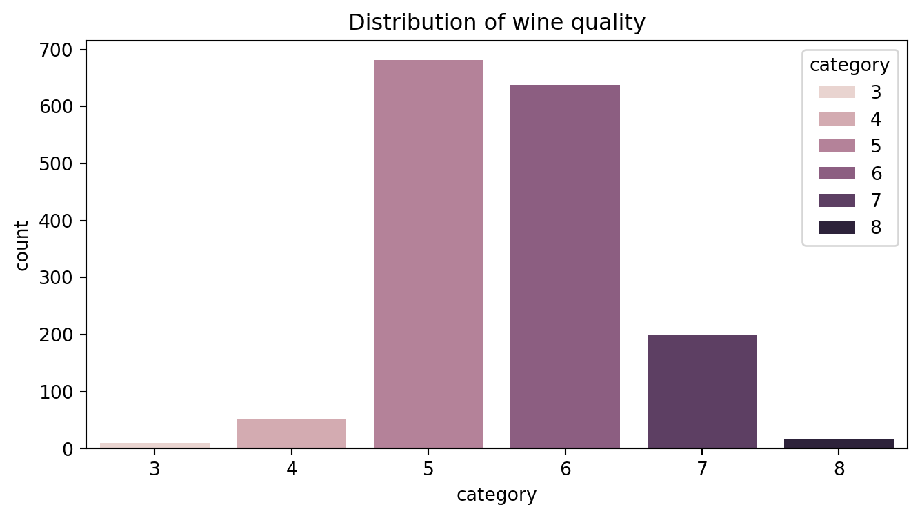
Example

• Task: Predicting target \(y\in\{1,2,\dots,M\}\) using its input \(\text{x}\in\mathbb{R}^d\).
• Example: Kaggle wine quality data.

Multinomial Logistic Regression

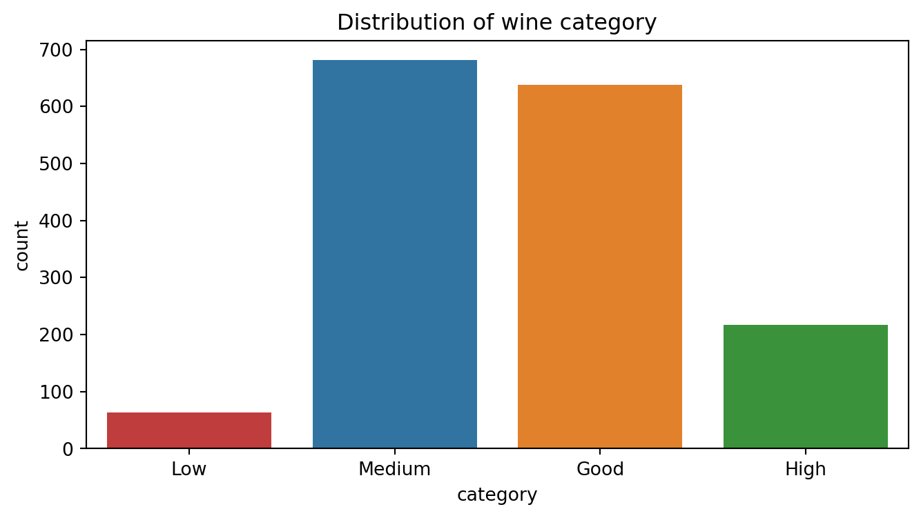
Example (modified)

• Task: Predicting target \(y\in\{1,2,\dots,M\}\) using its input \(\text{x}\in\mathbb{R}^d\).
• Example: Kaggle wine quality data.

Multinomial Logistic Regression

Model

• In this case, \(y\) takes \(M\) distinct values, it’s often encoded to be \(M\)-dimensional vector: \[y=k\Leftrightarrow p=(0,\dots,0,\underbrace{1}_{k\text{th index}},0,\dots,0)^T.\]
• The model also returns \(M\)-dimensional probability vector where index with highest probability is the predicted class.
• \(\text{Softmax}:\mathbb{R}^M\to\mathbb{S}_{M-1}=\{p_j\in[0,1]^M:\sum_{j=1}^Mp_j=1\}\) defined by \[\vec{z}\mapsto \vec{s}=\text{Softmax}(z)=\Big(\frac{e^{z_1}}{\sum_{j=1}^Me^{z_j}},\dots,\frac{e^{z_M}}{\sum_{j=1}^Me^{z_j}}\Big).\]
• It converts any \(M\)-dimensional vector \(\vec{z}\) to \(M\)-dimensional probability vector \(\vec{s}\).

Multinomial Logistic Regression

Model

• \(\text{Softmax}:\mathbb{R}^M\to\mathbb{S}_{M-1}=\{p_j\in[0,1]^M:\sum_{j=1}^Mp_j=1\}\) defined by \[\vec{z}\mapsto \vec{s}=\text{Softmax}(z)=\Big(\frac{e^{z_1}}{\sum_{j=1}^Me^{z_j}},\dots,\frac{e^{z_M}}{\sum_{j=1}^Me^{z_j}}\Big).\]

• Model: Given parameter matrix \(\color{green}{W}\) of size \(M\times d\) and intercept vector \(\color{green}{\vec{b}}\in\mathbb{R}^d\), the predicted probability of any input data \(\text{x}_i\in\mathbb{R}^d\) is defined by

\[\begin{align*}\color{red}{\hat{p}_i}&=\text{Softmax}(\color{green}{W}\text{x}_i+\color{green}{\vec{b}})\\ &=\text{Softmax}\begin{pmatrix} \color{green}{\begin{bmatrix}w_{11}& \dots & w_{1d}\\ w_{11}& \dots & w_{1d}\\ \vdots & \vdots & \vdots\\ w_{M1}& \dots & w_{Md}\end{bmatrix}}\begin{bmatrix}x_{i1}\\ x_{i2}\\ \vdots\\ x_{id}\end{bmatrix}+\color{green}{\begin{bmatrix}b_{1}\\ b_{2}\\ \vdots\\ b_{M}\end{bmatrix}}\end{pmatrix}=\color{red}{\begin{bmatrix}p_{i1}\\ p_{i2}\\ \vdots\\ p_{iM}\end{bmatrix}}\end{align*}\]

Multinomial Logistic Regression

Model

\[\begin{align*}\color{red}{\hat{p}_i}&=\text{Softmax}(\color{green}{W}\text{x}_i+\color{green}{\vec{b}})\\ &=\text{Softmax}\begin{pmatrix} \color{green}{\begin{bmatrix}w_{11}& \dots & w_{1d}\\ w_{11}& \dots & w_{1d}\\ \vdots & \vdots & \vdots\\ w_{M1}& \dots & w_{Md}\end{bmatrix}}\begin{bmatrix}x_{i1}\\ x_{i2}\\ \vdots\\ x_{id}\end{bmatrix}+\color{green}{\begin{bmatrix}b_{1}\\ b_{2}\\ \vdots\\ b_{M}\end{bmatrix}}\end{pmatrix}=\color{red}{\begin{bmatrix}p_{i1}\\ p_{i2}\\ \vdots\\ p_{iM}\end{bmatrix}}\end{align*}\]

Multinomial Logistic Regression

Cross-entropy loss

• We search for best possible parameters \(\color{green}{W}\in\mathbb{R}^{M\times d}\) and \(\color{green}{\vec{b}}\in\mathbb{R}^d\) by minimizing Cross Entropy loss defined below: \[\text{CEn}(W,\vec{b})=-\sum_{i=1}^n\sum_{m=1}^M\color{blue}{p_{im}}\log(\color{red}{\hat{p}_{im}}),\text{ where }\color{red}{\widehat{\text{p}}_i}=(\color{red}{\hat{p}_{i1}},\color{red}{\dots},\color{red}{\hat{p}_{iM}})\text{ is the predicted probability of }\color{blue}{\text{p}_i}.\]

Multinomial Logistic Regression

Gradient of Cross-Entropy

Optimizing Cross-entropy in Multinomial Logistic Regression

• Cross Entropy of any parameter \(\color{green}{W}\in\mathbb{R}^{M\times d}\) and \(\color{green}{\vec{b}}\in\mathbb{R}^d\): \(\text{CEn}(\color{green}{W},\color{green}{\vec{b}})=-\sum_{i=1}^n\sum_{m=1}^M\color{blue}{p_{im}}\log(\color{red}{\widehat{p}_{im}})\).
• Challenge: Show that
  • \(\nabla_{\color{green}{\vec{b}}} \text{CEn}(\color{green}{W},\color{green}{\vec{b}})=\sum_{i=1}^n\nabla_{\color{green}{\vec{b}}} \ell(\color{blue}{\text{p}_i},\color{red}{\hat{\text{p}}_i})=-\sum_{i=1}^n\underbrace{(\color{blue}{\text{p}_i}-\text{softmax}(\color{green}{W}\text{x}+\color{green}{\vec{b}}))}_{\in\mathbb{R}^d}\).
  • \(\nabla_{\color{green}{W}} \text{CEn}(\color{green}{W},\color{green}{\vec{b}})=\sum_{i=1}^n\nabla_{\color{green}{W}} \ell(\color{blue}{\text{p}_i},\color{red}{\widehat{p}_i})=-\sum_{i=1}^n\underbrace{(\color{blue}{\text{p}_i}-\color{red}{\widehat{\text{p}}_i})}_{\in\mathbb{R}^{d\times 1}}\underbrace{\text{x}_i^T}_{\in\mathbb{R}^{1\times d}}=\underbrace{(\color{red}{\widehat{P}}-\color{blue}{P})^TX}_{\in\mathbb{R}^{d\times d}}\), where

\[\begin{align*} \color{red}{\hat{P}}=\color{red}{\underbrace{\begin{bmatrix} \hat{p}_{11} &\dots & \hat{p}_{1d}\\ \vdots & \vdots & \vdots\\ \hat{p}_{n1} &\dots & \hat{p}_{nd} \end{bmatrix}}_{\text{Matrix of predicted probab}}}, \color{blue}{P}=\color{blue}{\underbrace{\begin{bmatrix} p_{11} &\dots & p_{1d}\\ \vdots & \vdots & \vdots\\ p_{n1} &\dots & p_{nd} \end{bmatrix}}_{\text{One-hot encoded matrix of $y_i$}}}\text{ and } X=\underbrace{\begin{bmatrix} x_{11} &\dots & x_{1d}\\ \vdots & \vdots & \vdots\\ x_{n1} &\dots & x_{nd} \end{bmatrix}}_{\text{Matrix of inputs $x_i$}} \end{align*}\]

Further reading: J. Chiang (2023) and K. Stratos (2018).

Multinomial Logistic Regression

In action: Kaggle wine quality data

df_wine.iloc[:,:-2].corr().round(3).style.background_gradient()

	fixed.acidity	volatile.acidity	citric.acid	residual.sugar	chlorides	free.sulfur.dioxide	total.sulfur.dioxide	density	pH	sulphates	alcohol
fixed.acidity	1.000000	-0.256000	0.672000	0.115000	0.094000	-0.154000	-0.113000	0.668000	-0.683000	0.183000	-0.062000
volatile.acidity	-0.256000	1.000000	-0.552000	0.002000	0.061000	-0.011000	0.076000	0.022000	0.235000	-0.261000	-0.202000
citric.acid	0.672000	-0.552000	1.000000	0.144000	0.204000	-0.061000	0.036000	0.365000	-0.542000	0.313000	0.110000
residual.sugar	0.115000	0.002000	0.144000	1.000000	0.056000	0.187000	0.203000	0.355000	-0.086000	0.006000	0.042000
chlorides	0.094000	0.061000	0.204000	0.056000	1.000000	0.006000	0.047000	0.201000	-0.265000	0.371000	-0.221000
free.sulfur.dioxide	-0.154000	-0.011000	-0.061000	0.187000	0.006000	1.000000	0.668000	-0.022000	0.070000	0.052000	-0.069000
total.sulfur.dioxide	-0.113000	0.076000	0.036000	0.203000	0.047000	0.668000	1.000000	0.071000	-0.066000	0.043000	-0.206000
density	0.668000	0.022000	0.365000	0.355000	0.201000	-0.022000	0.071000	1.000000	-0.342000	0.149000	-0.496000
pH	-0.683000	0.235000	-0.542000	-0.086000	-0.265000	0.070000	-0.066000	-0.342000	1.000000	-0.197000	0.206000
sulphates	0.183000	-0.261000	0.313000	0.006000	0.371000	0.052000	0.043000	0.149000	-0.197000	1.000000	0.094000
alcohol	-0.062000	-0.202000	0.110000	0.042000	-0.221000	-0.069000	-0.206000	-0.496000	0.206000	0.094000	1.000000

Multinomial Logistic Regression

In action: Target vs Inputs

sns.set(style="whitegrid")
_, axs = plt.subplots(2,3,figsize=(10,5))
i = 0
for var in df_wine.columns[:6]:
    sns.boxplot(df_wine, x="category", y=var, 
                hue="category", ax=axs[i//3, i%3],
                order=['Low', 'Medium', 'Good', 'High'])
    axs[i//3, i%3].set_title(f"Category vs {var}")
    i += 1
plt.tight_layout()
plt.show()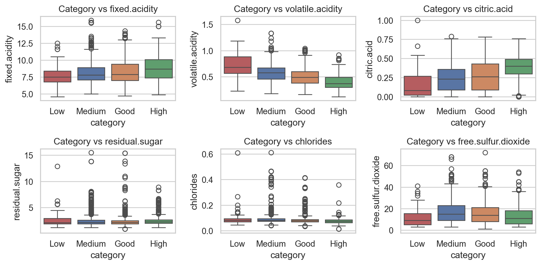

Multinomial Logistic Regression

In action: Target vs Inputs

from matplotlib.gridspec import GridSpec
fig = plt.figure(figsize=(10,5))

gs = GridSpec(4, 6)
axs = []
i = 0
for var in df_wine.columns[6:-2]:
    if i < 2:
        axs.append(fig.add_subplot(gs[:2, (2*i % 6):(2*i+2)%6]))
    elif i == 2:
        axs.append(fig.add_subplot(gs[:2, 4:]))
    elif i == 3:
        axs.append(fig.add_subplot(gs[2:, 1:3]))
    else:
        axs.append(fig.add_subplot(gs[2:, 3:5]))
    sns.boxplot(df_wine, x="category", y=var, 
                hue="category", ax=axs[-1],
                order=['Low', 'Medium', 'Good', 'High'])
    axs[-1].set_title(f"Category vs {var}")
    i += 1
plt.tight_layout()
plt.show()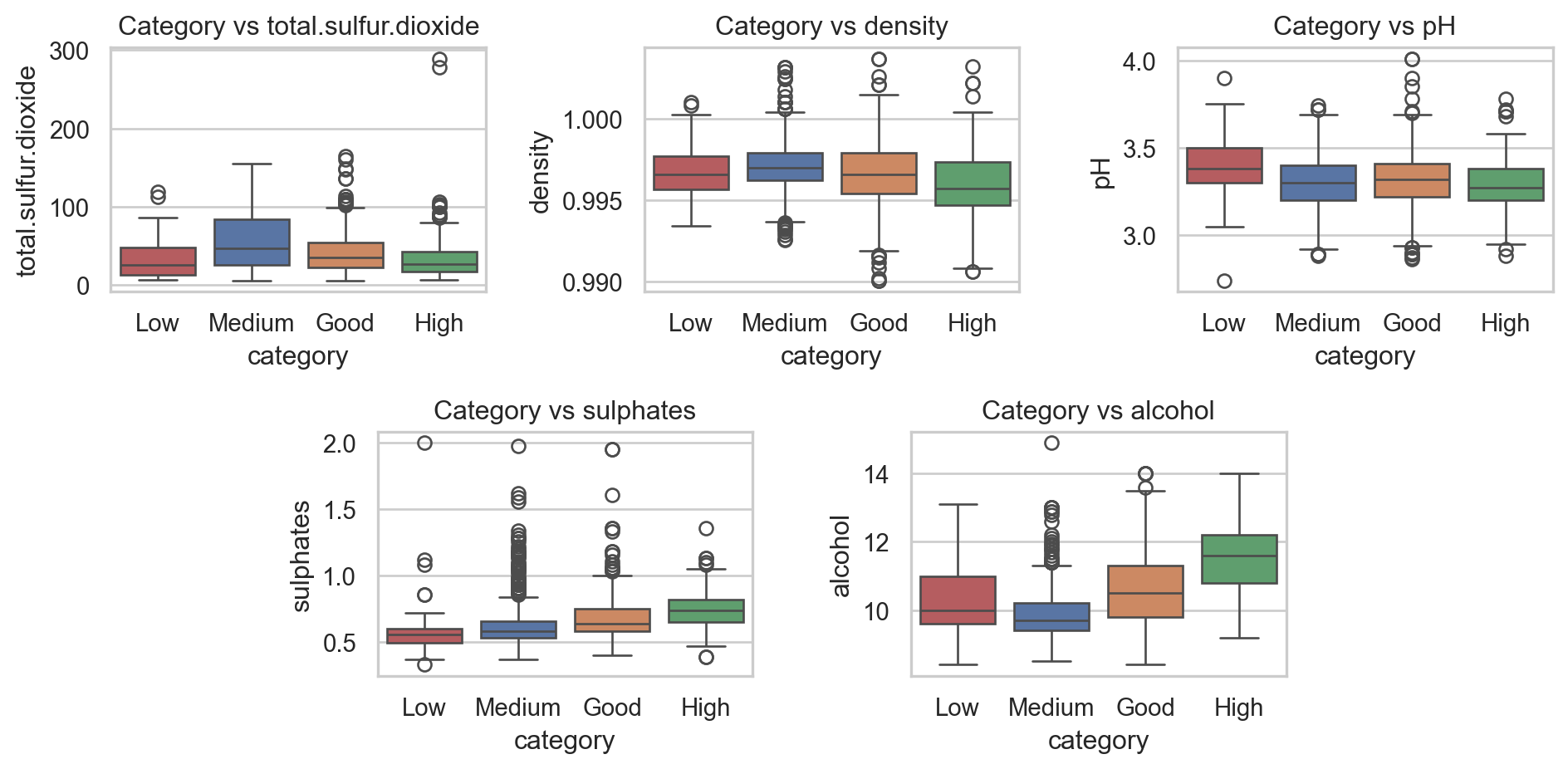

Multinomial Logistic Regression

In action: Kaggle wine quality data

Multinomial Logistic Regression

from sklearn.preprocessing import MinMaxScaler, PolynomialFeatures
from sklearn.model_selection import train_test_split
from sklearn.metrics import accuracy_score, balanced_accuracy_score, f1_score, recall_score, precision_score, log_loss, confusion_matrix, ConfusionMatrixDisplay
# Train test split
X_wine_train, X_wine_test, y_wine_train, y_wine_test = train_test_split(
    df_wine.iloc[:,:-2], df_wine['category'], test_size=0.25, 
    stratify=df_wine['category'], 
    random_state=42)
# Scaling data
scaler = MinMaxScaler()
# Fitting the model
X_wine_train = scaler.fit_transform(X_wine_train)
X_wine_test = scaler.transform(X_wine_test)
lgr = LogisticRegression(max_iter=300)
lgr_fit = lgr.fit(X_wine_train, y_wine_train)
y_hat_test1 = lgr_fit.predict(X_wine_test)
performance1 = pd.DataFrame( {
    'Acc': [accuracy_score(y_wine_test, y_hat_test1)], 
    'Balanced Acc': [balanced_accuracy_score(y_wine_test, y_hat_test1)], 
    'Precision': [precision_score(y_wine_test, y_hat_test1, average="macro")], 
    'Recall': [recall_score(y_wine_test, y_hat_test1, average="macro")], 
    'F1-score': [f1_score(y_wine_test, y_hat_test1, average="macro")] }, index=['Logit'])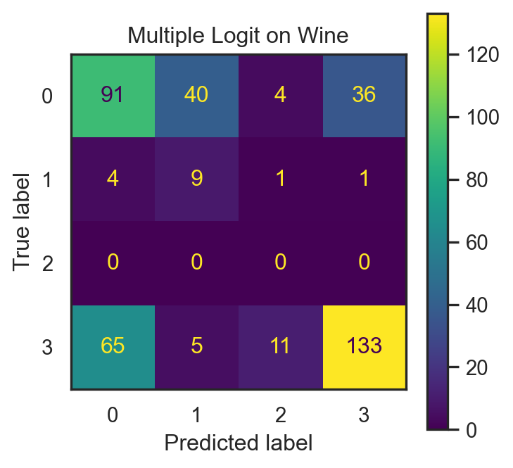

	Acc	Balanced Acc	Precision	Recall	F1-score
Logit	0.5825	0.379442	0.438415	0.379442	0.375857

Multinomial Logistic Regression

In action: Kaggle wine quality data

Multinomial Logistic Regression with Polynomial Features

degree = list(range(2,9,2))
# List to store all losses
poly_loss, poly_test_loss, test_loss = [], [], {}
for deg in degree:
    pf = PolynomialFeatures(degree=deg)
    X_poly = pf.fit_transform(X_wine_train)
    model = LogisticRegression(max_iter=300)
    score = -cross_val_score(model, X_poly, y_wine_train, cv=10, 
                scoring='neg_log_loss').mean()
    poly_loss.append(score)
    # Fit and predict
    model = model.fit(X_poly, y_wine_train)
    X_poly_test = pf.transform(X_wine_test)
    y_hat_test = model.predict(X_poly_test)
    prob = model.predict_proba(X_poly_test)
    poly_test_loss.append(log_loss(y_wine_test, prob))
    test_loss['Acc'] = [accuracy_score(y_wine_test, y_hat_test)]
    test_loss['Balanced Acc'] = [balanced_accuracy_score(y_wine_test, y_hat_test)]
    test_loss['Precision'] = [precision_score(y_wine_test, y_hat_test, average="macro")]
    test_loss['Recall'] = [recall_score(y_wine_test, y_hat_test, average="macro")]
    test_loss['F1-score'] = [f1_score(y_wine_test, y_hat_test, average="macro")]
    performance1 = pd.concat([performance1, pd.DataFrame(test_loss, index=[f'Poly {deg}'])])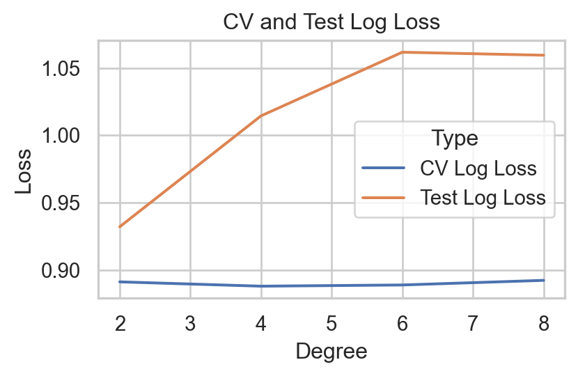

	Acc	Balanced Acc	Precision	Recall	F1-score
Logit	0.5825	0.379442	0.438415	0.379442	0.375857
Poly 2	0.5850	0.407704	0.708400	0.407704	0.426100
Poly 4	0.5925	0.432772	0.711266	0.432772	0.464086
Poly 6	0.5925	0.435747	0.707423	0.435747	0.467052
Poly 8	0.5925	0.435747	0.707353	0.435747	0.467121

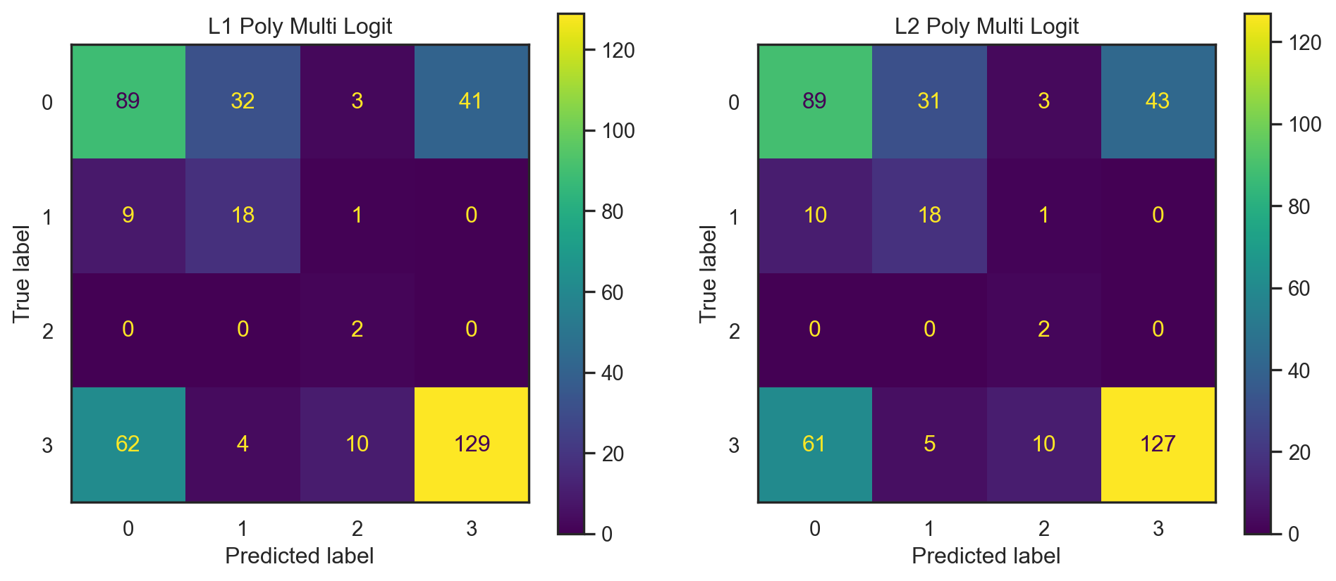
Multinomial Logistic Regression

In action: Kaggle wine quality data

\(L_2\) Regularized Multinomial Logistic Regression with Polynomial Features

deg_opt = np.argmin(performance1['F1-score'][1:])
pf = PolynomialFeatures(degree=degree[deg_opt])
X_poly = pf.fit_transform(X_wine_train)
X_poly_test = pf.transform(X_wine_test)
alphas = list(np.linspace(1e-5, 1, 30)) + list(np.linspace(1.01, 10, 30))
# List to store all losses
poly_loss, poly_test_loss, test_loss = [], [], {}
coefs = {f'alpha:{alp}': [] for alp in alphas}
for alp in alphas:
    model = LogisticRegression(penalty="l2", C=1/alp, max_iter=300)
    score = -cross_val_score(model, X_poly, y_wine_train, cv=10, 
                scoring='neg_log_loss').mean()
    poly_loss.append(score)
    # Fit and predict
    model = model.fit(X_poly, y_wine_train)
    y_hat_test = model.predict(X_poly_test)
    coefs[f'alpha:{alp}'] = model.coef_[0]
    prob = model.predict_proba(X_poly_test)
    poly_test_loss.append(log_loss(y_wine_test, prob))
    test_loss['Acc'] = [accuracy_score(y_wine_test, y_hat_test)]
    test_loss['Balanced Acc'] = [balanced_accuracy_score(y_wine_test, y_hat_test)]
    test_loss['Precision'] = [precision_score(y_wine_test, y_hat_test, average="macro")]
    test_loss['Recall'] = [recall_score(y_wine_test, y_hat_test, average="macro")]
    test_loss['F1-score'] = [f1_score(y_wine_test, y_hat_test, average="macro")]
    performance1 = pd.concat([performance1, pd.DataFrame(test_loss, index=[f'L2-Alp:{alp}'])])

Multinomial Logistic Regression

In action: Kaggle wine quality data

\(L_1\) Regularized Multinomial Logistic Regression with Polynomial Features

alphas = list(np.linspace(1e-5, 1, 30)) + list(np.linspace(1.01, 10, 30))
# List to store all losses
poly_loss, poly_test_loss, test_loss = [], [], {}
coefs = {f'alpha:{alp}': [] for alp in alphas}
for alp in alphas:
    model = LogisticRegression(penalty="l1", solver='saga', C=1/alp, max_iter=300)
    score = -cross_val_score(model, X_poly, y_wine_train, cv=10, 
                scoring='neg_log_loss').mean()
    poly_loss.append(score)
    # Fit and predict
    model = model.fit(X_poly, y_wine_train)
    coefs[f'alpha:{alp}'] = model.coef_[0]
    X_poly_test = pf.transform(X_wine_test)
    y_hat_test = model.predict(X_poly_test)
    prob = model.predict_proba(X_poly_test)
    poly_test_loss.append(log_loss(y_wine_test, prob))
    test_loss['Acc'] = [accuracy_score(y_wine_test, y_hat_test)]
    test_loss['Balanced Acc'] = [balanced_accuracy_score(y_wine_test, y_hat_test)]
    test_loss['Precision'] = [precision_score(y_wine_test, y_hat_test, average="macro")]
    test_loss['Recall'] = [recall_score(y_wine_test, y_hat_test, average="macro")]
    test_loss['F1-score'] = [f1_score(y_wine_test, y_hat_test, average="macro")]
    performance1 = pd.concat([performance1, pd.DataFrame(test_loss, index=[f'L1-Alp:{alp}'])])

Multinomial Logistic Regression

Summary

	Acc	Balanced Acc	Precision	Recall	F1-score
Logit	0.5825	0.379442	0.438415	0.379442	0.375857
Poly 2	0.5850	0.407704	0.708400	0.407704	0.426100
Poly 4	0.5925	0.432772	0.711266	0.432772	0.464086
Poly 6	0.5925	0.435747	0.707423	0.435747	0.467052
Poly 8	0.5925	0.435747	0.707353	0.435747	0.467121
L2-Alp:0.138	0.5900	0.440411	0.695612	0.440411	0.470734
L1-Alp:0.724	0.5950	0.443352	0.702880	0.443352	0.474235

Multinomial Logistic Regression

Summary

Pros & Cons

Pros

• Simplicity: It’s easy to understand and implement.
• Efficiency: It’s not so computationally expensive, making it suitable for large datasets.
• Interpretability: It converts relative distances from input data to boundary decision into probabilities, which can be meaningfully interpreted.
• No Scaling Required: It doesn’t require input features to be scaled or standardized (you can also tranform for efficient computation).
• Works Well with Linearly Separable Data: Performs well when the data is linearly separable.

Cons

• Assumes Linearity: Assumes a linear relationship between the independent variables and the log-odds of the dependent variable.
• Sensitivity to Outliers: Outliers can affect the model’s performance and accuracy.
• Overfitting: Can overfit if the dataset has a large number of features compared to the number of observations.
• Limited to Binary Outcomes: Standard logistic regression is designed for binary classification and may not perform as well with multiclass classification problems.
• Assumes Independence of Errors: Assumes that the observations are independent of each other and that there is no multicollinearity among predictors.

🥳 It’s party time 🥂

📋 View party menu here: Party 2 Menu.

🫠 Download party invitation here: Party 2 Invitation Letter.