import pandas as pd # Import pandas packageimport seaborn as sns # Package for beautiful graphsimport matplotlib.pyplot as plt # Graph managementsns.set(style="whitegrid") # Set grid background# path = "https://gist.githubusercontent.com/curran/4b59d1046d9e66f2787780ad51a1cd87/raw/9ec906b78a98cf300947a37b56cfe70d01183200/data.tsv" # The data can be found in this linkdf0 = pd.read_csv(path) # Import it into Pythondf0.head(5) # Randomly select 4 points
eruptions
waiting
0
3.600
79
1
1.800
54
2
3.333
74
3
2.283
62
4
4.533
85
Code
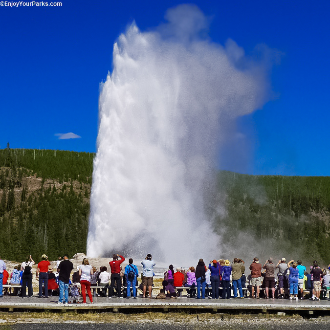
plt.figure(figsize=(5,3.2)) # Define figure sizesns.scatterplot(df0, x="waiting", y="eruptions") # Create scatterplotplt.title("Old Faithful data from Yellowstone National Park, US", fontsize=10) # Titleplt.suptitle("Eruptions vs waiting times", fontsize=13, y=1) # Subtitleplt.show()
The longer the wait, the longer duration of the eruption.
import plotly.express as pxfig = px.scatter_3d(df1, x="youtube", y="facebook", z="sales", size="newspaper", color="newspaper", size_max=40)camera =dict(eye=dict(x=1, y=-1, z=1.2))fig.update_layout(title="Sales as a function of all ads", width=550, height=350, scene_camera=camera)
Increasing ads seems to boost sales!
Our Motivational Quote Today
“Where there is data smoke, there is business fire.” — Thomas Redman
Predict \(y\) using only a single input \(\text{x}\in\mathbb{R}\).
Model: \(\underbrace{\hat{y}}_{\text{predicted eruption}}=\beta_0+\beta_1\underbrace{\text{x}}_{\text{waiting}}\) for \(\beta_0,\beta_1\in\mathbb{R}\).
Simple Linear Regression (SLR)
Residual Sum of Squares: \(\begin{align*}
\text{RSS}&=\sum_{i=1}^n(\color{red}{y_i-\hat{y}_i})^2\\
&=\sum_{i=1}^n(\color{red}{y_i-\beta_0-\beta_1x_i})^2
\end{align*}\)
Ordinary Least Squares (OLS): The best-fitted line minimizes TSS.
Model: \(\underbrace{\hat{y}}_{\text{predicted eruption}}=\beta_0+\beta_1\underbrace{\text{x}}_{\text{waiting}}\) for \(\beta_0,\beta_1\in\mathbb{R}\).
Simple Linear Regression (SLR)
Simple Linear Regression (SLR)
Optimal Least-square line
Optimal Least-Square Line
Optimal line: \(\hat{y}=\hat{\beta}_0+\hat{\beta}_1\text{x}\) where
\[\begin{align}
\hat{\beta}_1&=\frac{\sum_{i=1}^n(\text{x}_i-\overline{\text{x}}_n)(y_i-\overline{y}_n)}{\sum_{i=1}^n(\text{x}_i-\overline{\text{x}}_n)^2}=\frac{\text{Cov}(X,Y)}{\text{V}(X)}\\
\hat{\beta}_0&=\overline{y}_n-\hat{\beta}_1\overline{\text{x}}_n\end{align},
\] with
\(\overline{\text{x}}_n=\frac{1}{n}\sum_{i=1}^n\text{x}_i\) and \(\overline{y}_n=\frac{1}{n}\sum_{i=1}^ny_i\) be the average/mean of \(X\) and \(Y\) resp.
\(\text{Cov}(X,Y)=\frac{1}{n}\sum_{i=1}^n(\text{x}_i-\overline{\text{x}}_n)(y_i-\overline{y}_n)\) be the “covariance” between \(X\) & \(Y\).
\(\text{V}(X)=\frac{1}{n}\sum_{i=1}^n(\text{x}_i-\overline{\text{x}}_n)^2\) be the “variance” of \(X\).
Simple Linear Regression (SLR)
Apply on marketing data
Simple Linear Regression (SLR)
Apply on marketing data (cont.)
Code
from sklearn.linear_model import LinearRegression # import modellr = LinearRegression() # initiate modelx_train, y_train = df1[['youtube']], df1['sales'] # training input-targetlr = lr.fit(x_train, y_train) # build model = esimate coefficients# Training data and fitted linepred_train = lr.predict(x_train)# Figuresfig_market2 = go.Figure(go.Scatter(x=x_train.youtube, y=y_train, mode="markers", name="Training data"))fig_market2.add_trace(go.Scatter(x=x_train.youtube, y=pred_train, mode="lines+markers", name=f"<br>Train prediction<br> Sale={np.round(lr.coef_,2)[0]}youtube+{np.round(lr.intercept_,2)}"))fig_market2.update_layout(title="Sales vs youtube", xaxis=dict(title="youtube"), yaxis=dict(title="sales"), width=600, height=400)fig_market2.show()
Simple Linear Regression (SLR)
Model Diagnostics (judging the model)
R-squared (coefficient of determination)\[R^2=1-\frac{\text{RSS}}{\text{TSS}}=1-\frac{\sum_{i=1}(y_i-\hat{y}_i)^2}{\sum_{i=1}(y_i-\overline{y}_n)^2}=\frac{\text{V}(\hat{Y})}{\text{V}(Y)}.\]
Example: \(R^2=\) 0.612 in our model.
Interpretation: The model (youtube) can capture around 61.0% of the variation of the target (sales).
Simple Linear Regression (SLR)
Model Diagnostics (judging the model)
Residuals: \(e_i=y_i-\hat{y}_i\sim{\cal N}(0,\sigma^2)\) for some \(\sigma>0\).
Symmetric around \(0\) & do NOT depend on \(\text{x}_i\) nor \(y_i\).
Coefficient \(\beta_1=\) 0.048 indicates that Sales is expected to increase (or decrease) by 0.048 units for every \(1\) unit increase (or decrease) in YouTube ads.
R-squared: Represents the proportion of the target’s variation captured by the model.
Residual: In a good model, the residuals should be random noise, indicating the model has captured most of the information from the target.
Marketing example:
The amount in ad on YouTube alone can explain around \(61\)% (R-squared) of the variation in sales.
However, the residuals still contain patterns (large errors at small and large predicted sales), suggesting the model can be improved.
Multiple Linear Regression
Correlation Matrix
Pearson’s correlation coefficient
Correlation between two columns \(X_1\) and \(X_2\): \[r=r_{X_1,X_2}=\frac{\sum_{i=1}^n(x_{i1}-\overline{x}_{1})(x_{i2}-\overline{x}_{2})}{\sqrt{\left(\sum_{i=1}^n(x_{i1}-\overline{x}_{1})^2\right)\left(\sum_{i=1}^n(x_{i2}-\overline{x}_{2})^2\right)}}\]
\(-1\leq r\leq 1\) for any pair \(X_1\) and \(X_2\).
If \(r\approx 1\), then \(X_1\) and \(X_2\) are positively correlated (one ↗️, another ↗️).
If \(r\approx -1\), then \(X_1\) and \(X_2\) are negatively correlated (one ↗️, another ↘️)
If \(r\approx 0\), then \(X_1\) and \(X_2\) are decorrelated (no pattern or relation).
It helps identifying informative/useful inputs for the building models.
It also helps identifying redundant (strongly correlated) inputs.
Note: Correlation does not imply causation; it only indicates a relationship, not a cause-and-effect link.
Correlation matrix
Examples
Correlation Matrix
Example: marketing data
cor = df1.corr() # df1 is the marketing datacor.style.background_gradient()
youtube
facebook
newspaper
sales
youtube
1.000000
0.054809
0.056648
0.782224
facebook
0.054809
1.000000
0.354104
0.576223
newspaper
0.056648
0.354104
1.000000
0.228299
sales
0.782224
0.576223
0.228299
1.000000
YouTube is strongly correlated with target Sales and is most useful for building models, followed by Facebook and Newspaper.
Facebook and Newspaper have a significantly larger correlation with each other than with YouTube.
Multiple Linear Regression (MLR)
Predict \(y\) using more than one input \(\text{x}\in\mathbb{R}^d\).
Model: \(\underbrace{\hat{y}}_{\text{Sales}}=\beta_0+\beta_1\underbrace{x_1}_{\text{FB}}+\beta_2\underbrace{x_2}_{\text{NP}}\) for \(\beta_0,\beta_1,\beta_2\in\mathbb{R}\).
A better criterion, Adjusted R-squared: \[R^2_{\text{adj}}=1-\frac{n-1}{n-d-1}(1-R^2).\] Here, \(n\) is the number of obs, \(d\) is the number of inputs.
For our built model: \(R^2=\) 0.333 and \(R^2_{\text{adj}}=\) 0.326 (not so good!).
\(R^2_{\text{adj}}\) is always smaller than \(R^2\). A large \(R^2\) with only a slight decrease in \(R^2_{\text{adj}}\) indicates a good MLR model.
Rough interpretion, \(\beta_1=\) 0.199 indicates that if facebook ad is increased (or decreased) by \(1\) unit, sales is expected to increase (or decrease) by 0.199 units.
Explain: \(\beta_2=\) 0.007.
\(R^2=\) 0.333 indicates that around \(33.33\)% variation of the sales can be explained by ads on Facebook and Newspaper together, which is not enough to be a good model!
A slight decrease in \(R^2_{\text{adj}}=\) 0.326 suggests that the information provided by both variables is not redundant for explaining sales.
There are some large negative values of residuals, indicating that the model overestimated some actual target especially around large sales.
What’s next?
Use standardized inputs: \(\text{x}_i\to \tilde{\text{x}}_i=\frac{\text{x}_i-\overline{\text{x}}_i}{\hat{\sigma}_{\text{x}_i}}\)
Overfitting happens when a model learns the training data too well, capturing noise and fluctuations rather than the underlying pattern.
It fits the training data almost perfectly, but fails to generalize to new, unseen data.
Complex models (high-degree poly. features) often overfit the data.
Overcoming overfitting
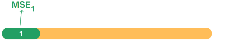
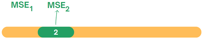
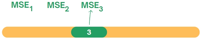
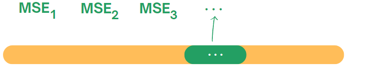
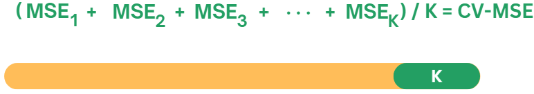
\(K\)-fold Cross-Validation
It ensures that the model performs well on different subsets.
The most common technique to overcome overfitting.
Tuning Polynomial degree Using \(K\)-fold Cross-Validation
from sklearn.preprocessing import PolynomialFeaturesfrom sklearn.linear_model import LinearRegression as LRfrom sklearn.model_selection import cross_val_score# DataX, y = market[["youtube"]], market['sales']# List of all degrees to search overdegree =list(range(1,11))# List to store all lossesloss = [] for deg in degree: pf = PolynomialFeatures(degree=deg) X_poly = pf.fit_transform(X) model = LR() score =-cross_val_score(model, X_poly, y, cv=5, scoring='neg_mean_squared_error').mean() loss.append(score)
overcoming overfitting
Regularization
Another approach is to controll the magnitude of the coefficients.
It often works well for SLR, MLR and Polynomial Regression…
Objective: Search for \(\vec{\beta}=[\beta_0,\dots,\beta_d]\) minimizing the following loss function for some \(\color{green}{\alpha}>0\): \[{\cal L}_{\text{ridge}}(\vec{\beta})=\color{red}{\underbrace{\sum_{i=1}^n(y_i-\widehat{y}_i)^2}_{\text{RSS}}}+\color{green}{\alpha}\color{blue}{\underbrace{\sum_{j=0}^{d}\beta_j^2}_{\text{Magnitude}}}.\]
Recall: SLR & MLR seek to minimize only RSS.
Overcoming overfitting
Regularization: Ridge Regression
Large \(\color{green}{\alpha}\Rightarrow\) strong penalty \(\Rightarrow\) small \(\vec{\beta}\).
Small \(\color{green}{\alpha}\Rightarrow\) weak penalty \(\Rightarrow\) freer \(\vec{\beta}\).
🔑 Objective: Learn the best \(\color{green}{\alpha}>0\).
How to find a suitable regularization strength \(\color{green}{\alpha}\)?
Overcoming overfitting
Regularization: Ridge Regression
Tuning Regularization Stregnth \(\color{green}{\alpha}\) Using \(K\)-fold Cross-Validation
from sklearn.preprocessing import PolynomialFeaturesfrom sklearn.linear_model import Ridgefrom sklearn.model_selection import cross_val_score# DataX, y = market[["youtube"]], market['sales']poly = PolynomialFeatures(degree=8)X_poly = poly.fit_transform(X)# List of all degrees to search overalphas =list(np.linspace(0.01, 3, 30)) +list(np.linspace(3.1, 20000, 30))# List to store all lossesloss = []coefficients = {f'alpha={alpha}': [] for alpha in alphas}for alp in alphas: model = Ridge(alpha=alp) score =-cross_val_score(model, X_poly, y, cv=5, scoring='neg_mean_squared_error').mean() loss.append(score)# Fit model.fit(X_poly, y) coefficients[f'alpha={alp}'] = model.coef_
Overcoming overfitting
Regularization: Ridge Regression
Tuning Regularization Stregnth \(\color{green}{\alpha}\) Using \(K\)-fold Cross-Validation
Overcoming overfitting
Regularization: Ridge Regression
Tuning Regularization Stregnth \(\color{green}{\alpha}\) Using \(K\)-fold Cross-Validation
Overcoming overfitting
Regularization: Ridge Regression
Pros
It works well when there are inputs that are approximately linearly related with the target.
It helps stabilize the estimates when inputs are highly correlated.
It can prevent overfitting.
It is effective when the number of inputs exceeds the number of observations.
Cons
It does not work well when the input-output relationships are highly non-linear.
It may introduce bias into the coefficient estimates.
Objective: Search for \(\vec{\beta}=[\beta_0,\dots,\beta_d]\) minimizing the following loss function for some \(\color{green}{\alpha}>0\): \[{\cal L}_{\text{lasso}}(\vec{\beta})=\color{red}{\underbrace{\sum_{i=1}^n(y_i-\widehat{y}_i)^2}_{\text{RSS}}}+\color{green}{\alpha}\color{blue}{\underbrace{\sum_{j=0}^{d}|\beta_j|}_{\text{Magnitude}}}.\]
Overcoming overfitting
Regularization: Lasso Regression
Large \(\color{green}{\alpha}\Rightarrow\) strong penalty \(\Rightarrow\) small \(\vec{\beta}\).
Small \(\color{green}{\alpha}\Rightarrow\) weak penalty \(\Rightarrow\) freer \(\vec{\beta}\).
🔑 Objective: Learn the best \(\color{green}{\alpha}>0\).
Tuning Regularization Stregnth \(\color{green}{\alpha}\) Using \(K\)-fold Cross-Validation
Overcoming overfitting
Regularization: Lasso Regression
Pros
Lasso inherently performs feature selection when increasing regularization parameter \(\alpha\) (less important variables are forced to be completely \(0\)).
It works well when there are many inputs (high-dimensional data) and some highly correlated with the target.
It can handle collinearities (many redundant inputs).
It can prevent overfitting and offers high interpretability.
Cons
It does not work well when the input-output relationships are highly non-linear.
It may introduce bias into the coefficient estimates.
It is sensitive to the scale of the data, so proper scaling of predictors is crucial before applying the method.