
II. Bivariate Analysis


Exploratory Data Analysis & Unsupervised Learning


Lecturer: Dr. HAS Sothea

helpful resources

1 Motivation

1.1 Motivation

Gapminder dataset (1704, 5)

  • This dataset captures the world’s evolution from \(1952\) to \(2007\).
  • Now, take a look at the data from year \(2007\).
Code
from gapminder import gapminder
import numpy as np
data2007 = gapminder[gapminder.year == 2007]  # filter to year 2007
data2007.iloc[:5,:].drop(columns=['year']).style.hide()
country continent lifeExp pop gdpPercap
Afghanistan Asia 43.828000 31889923 974.580338
Albania Europe 76.423000 3600523 5937.029526
Algeria Africa 72.301000 33333216 6223.367465
Angola Africa 42.731000 12420476 4797.231267
Argentina Americas 75.320000 40301927 12779.379640
Code
quan_vars = ["pop", "lifeExp", "gdpPercap"]
data2007[quan_vars].describe().transpose().drop(columns=["count", "25%", "75%"]).transpose()
pop lifeExp gdpPercap
mean 4.402122e+07 67.007423 11680.071820
std 1.476214e+08 12.073021 12859.937337
min 1.995790e+05 39.613000 277.551859
50% 1.051753e+07 71.935500 6124.371108
max 1.318683e+09 82.603000 49357.190170

Gapminder dataset (1704, 5)

  • This dataset captures the world’s evolution from \(1952\) to \(2007\).
  • Now, take a look at the data from year \(2007\) (visualization).
Code
from plotly.subplots import make_subplots
import plotly.graph_objects as go
fig = make_subplots(rows=1, cols=3, 
              subplot_titles=("Boxplot of pop", "Violinplot of lifeExp", "Histogram of GDP Per Capita"))
fig.add_trace(go.Box(y=data2007['pop'], name="pop"), col=1, row=1)
fig.add_trace(go.Violin(y=data2007['lifeExp'], name="lifeExp"), row=1, col=2)
fig.add_trace(go.Histogram(x=data2007['gdpPercap'],
              name="gdpPercap"), row=1, col=3)
fig.update_layout(height=280, width=900)
fig.update_yaxes(type="log", row=1, col=1)
fig.update_xaxes(title="Population", row=1, col=1)
fig.update_xaxes(title="Life Expectancy", row=1, col=2)
fig.update_xaxes(title="GDP Per Capita", row=1, col=3)
fig.show()

Objective

  • What indicators and graphs shall be used to detect relationship between different type of columns?
    • Case 1: Quantitative vs Quantitative.
    • Case 2: Quantitative vs Categorical.
    • Case 3: Categorical vs Categorical.

2 Bivariate Analysis

2.1 Quantitative vs Quantitative

Indicator: Covariance

  • If \(X=[\text{x}_1,\text{x}_2,...,\text{x}_n]\) is a quan. column:
    • Mean/average: \(\overline{\text{x}}=\displaystyle\frac{1}{n}\sum_{i=1}\text{x}_i\).
    • Variance: \(V(X)=\displaystyle\frac{1}{n-1}\sum_{i=1}^n(\text{x}_i-\overline{x})^2.\)
    • Standard deviation: \(\hat{\sigma}=\sqrt{V(X)}\).
  • If \(Y=[\text{y}_1,\text{y}_2,\dots,\text{y}_n]\) is an other quan. column, the covaraince between \(X\) and \(Y\):

\[\text{Cov}(X,Y)=\frac{1}{n-1}\sum_{i=1}(\text{x}_i-\overline{x})(\text{y}_i-\overline{y}).\]

Code
import plotly.express as px
df = px.data.tips()
fig = px.scatter(df, y="tip", x="total_bill", color="sex", hover_data=df.columns)
fig.update_layout(width=380, height=250, title="Tips vs total bill & gender")
fig.show()
tip total_bill sex
0 1.01 16.99 Female
1 1.66 10.34 Male
2 3.50 21.01 Male

Indicator: Covariance

  • Covariance between quan. columns \(X\) & \(Y\):

\[\text{Cov}(X,Y)=\frac{1}{n-1}\sum_{i=1}(\text{x}_i-\overline{x})(\text{y}_i-\overline{y}).\]

  • It determines tendency/direction of linear relationship between \(X\) and \(Y\).
    • Positive: change in the same direction.
    • Negative: change in opposite direction.
Code
fig.update_layout(title=f"Tips vs total bill (Cov = {float(np.cov(df['tip'].values, df['total_bill'].values).round(2)[0,1])}) & gender ")
fig.update_layout(width=380, height=260, title="Tips vs total bill & gender")
fig.add_annotation(
    x=20, y=8, showarrow=False, font=dict(size=12), 
    text=f"Cov = {float(np.cov(df['tip'].values, df['total_bill'].values).round(2)[0,1])}"
)
fig.show()
tip total_bill sex
0 1.01 16.99 Female
1 1.66 10.34 Male
2 3.50 21.01 Male
3 3.31 23.68 Male
4 3.61 24.59 Female

It’s hard to interpret the value of covariance as it can be large or small according to the scale of \(X\) and \(Y\).

Indicator: Pearson Correlation Coefficient

  • Pearson correlation between two quantitative columns \(X\) and \(Y\): \[r=r_{X,Y}=\frac{\sum_{i=1}^n(\text{x}_{i}-\overline{x})(\text{y}_{i}-\overline{y})}{\sqrt{\left(\sum_{i=1}^n(x_{i}-\overline{x})^2\right)\left(\sum_{i=1}^n(x_{i}-\overline{y})^2\right)}}=\frac{\text{Cov}(X,Y)}{s_Xs_Y}.\]
  • It quantifies the linear relationship/tendency between the two variables.
    • For any pair \(X\) & \(Y\) one has \(-1\leq r\leq 1\).
    • \(r\approx 1\): \(X\) & \(Y\) are positively linearly correlated (upward trend).
    • \(r\approx -1\): \(X\) & \(Y\) are negatively linearly correlated (downward trend).
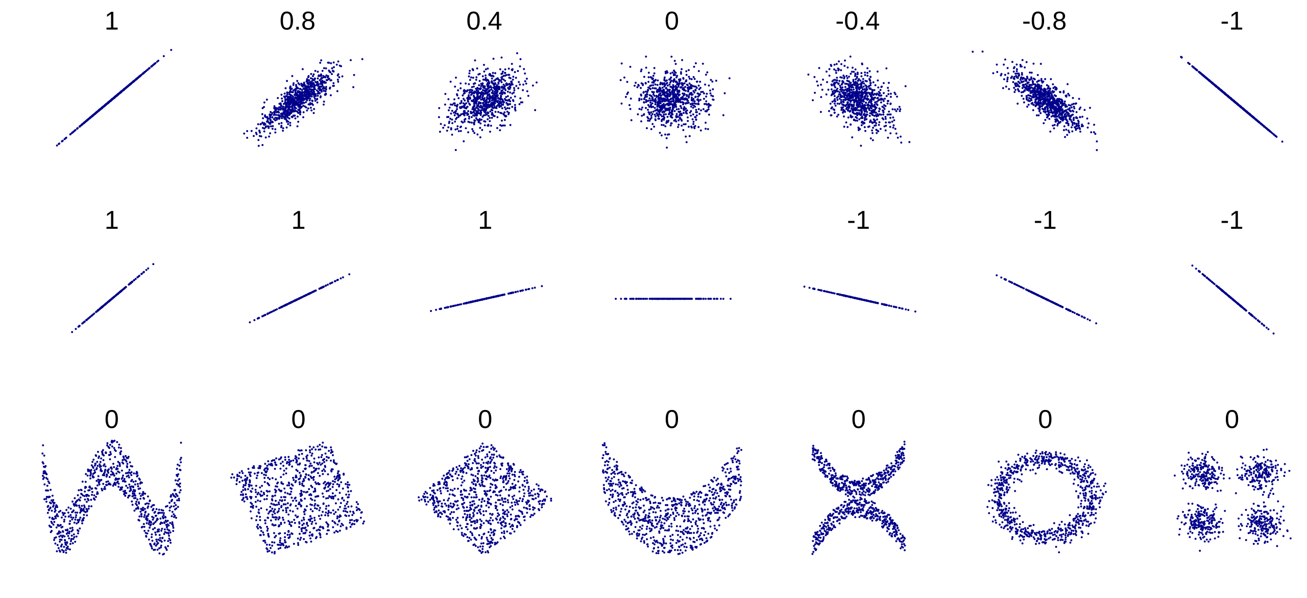
    • \(r\approx 0\): \(X\) & \(Y\) are decorrelated (no tendency) OR interrupted by noise.
  • For predictive analysis:
    • It helps identifying informative/useful inputs for the (linear) models.
    • It also helps identifying redundant (strongly correlated) inputs.
  • Correlation indicates tendency but NOT a cause-and-effect link [Read here].
  • For tip example: \(\text{Corr}(\text{tip}, \text{bill})=\) 0.676.

Indicator: Pearson Correlation Coefficient

  • Different examples of correlation between two variables:
Fig 1: Correlation examples. Source: https://en.wikipedia.org/wiki/Correlation.

Indicator: Pearson Correlation Matrix

  • To detect tendency of linear relationship between many quantitative columns, Pearson correlation matrix is a common tool to use.
  • It highlights the strongly linearly correlated pairs.
  • Consider Pearson corr. matrix on Gapminder in 2007:
cor = data2007[["gdpPercap", "lifeExp", "pop"]]\
    .corr()
cor.style.background_gradient(cmap='Accent')
  gdpPercap lifeExp pop
gdpPercap 1.000000 0.678662 -0.055676
lifeExp 0.678662 1.000000 0.047553
pop -0.055676 0.047553 1.000000
  • LifeExp and GDP appear to be positively related.
  • Population may be decorrelated with the other two columns.

2.2 Quan./Ordi. vs Quan./Ordi.

Indicator: Spearman’s Rank Correlation

  • Pearson correlation is sensitive to outliers (Lab 2) and does not capture non-linear relationship between quantitaive columns.
  • It is not sutiable for ordinal data (likert scale, for example).
  • Spearman’s Rank Correlation overcomes these limitations by measuring the strength and direction of the monotonic relationship between two variables, regardless of their distribution or the presence of outliers.
  • It is defined by:

\[\rho_{\color{blue}{X},\color{red}{Y}}=r_{R[{\color{blue}{X}}],R[{\color{red}{Y}}]}=\frac{\text{Cov}(R[{\color{blue}{X}}],R[{\color{red}{Y}}])}{s_{R[{\color{blue}{X}}]},s_{R[{\color{red}{Y}}]}}=1-\frac{6\sum_{i=1}^nd_i^2}{n(n^2-1)},\]

where \(R[{\color{blue}{\text{x}_i}}]\) and \(R[{\color{red}{\text{y}_i}}]\) be the rank of observations \(\color{blue}{\text{x}_i}\) and \(\color{red}{\text{y}_i}\) in their own list, and \(d_i=R[{\color{blue}{\text{x}_i}}]-R[{\color{red}{\text{y}_i}}]\) be the distance in rank of observation \(i\)-th.

Spearman’s Rank Correlation is large when most of the ranks of the two variables match.

Indicator: Spearman’s Rank Correlation

  • Example: \(X=[1,3,2,5,4]\) and \(Y=[0.1,1,0.2,1000,1.5]\)

Pearson correlation

  • \(\overline{X}=\color{red}{4}\) and \(\overline{Y}=\color{blue}{200.56}\).
  • \(s_X=\sqrt{\frac{(1-{\color{red}{4}})^2+(3-{\color{red}{4}})^2+\dots+(4-{\color{red}{4}})^2}{5-1}}=\color{red}{1.58}\)
    \(s_Y=\sqrt{\frac{(0.1-{\color{blue}{200.56}})^2+\dots+(1.5-{\color{blue}{200.56}})^2}{5-1}}=\color{blue}{446.9}\).
  • \(r_{X,Y}=\frac{(1-{\color{red}{4}})(0.1-{\color{blue}{200.56}})+\dots+(4-{\color{red}{4}})(1.5-{\color{blue}{200.56}})}{(\color{red}{1.58})(\color{blue}{446.9})}=\color{purple}{0.71}.\)

Spearman correlation

  • \(R[X]=[1,3,2,5,4]\) & \(R[Y]=[1,3,2,5,4]\).
  • All \(d_i=0\) therefore \(\rho_{X,Y}=1-\frac{6\sum_{i}d_i^2}{5(5^2-1)}=\color{purple}{1}\).
  • Pearson (Gapminder, 2007):
cor = data2007[["gdpPercap", "lifeExp", "pop"]].corr()
cor.style.background_gradient(cmap='Accent')
  gdpPercap lifeExp pop
gdpPercap 1.000000 0.678662 -0.055676
lifeExp 0.678662 1.000000 0.047553
pop -0.055676 0.047553 1.000000
  • Spearman (Gapminder, 2007):
cor = data2007[["gdpPercap", "lifeExp", "pop"]].corr("spearman")
cor.style.background_gradient(cmap='Accent')
  gdpPercap lifeExp pop
gdpPercap 1.000000 0.856590 -0.064588
lifeExp 0.856590 1.000000 0.003355
pop -0.064588 0.003355 1.000000

Summary

Aspect Pearson Spearman
Type Parametric Non-parametric
Measure Linear relationship Monotonic relationship
Data Type Numerical Ordinal or Numerical
Outliers Sensitive to outliers Less sensitive to outliers
Range \([-1,1]\) \([-1,1]\)
Interpretation \(\approx\) 1: Perfect positive linear relationship
\(\approx\) -1: Perfect negative linear relationship
\(\approx\) 0: No linear trend or interrupted by noise
\(\approx\) 1: Perfect increasing monotonic relationship
\(\approx\) -1: Perfect decreasing monotonic relationship
\(\approx\) 0: No monotonic relationship at all

Visualization: Scatterplot

  • Let’s visualize: gdpPercap wih lifeExp & pop.
Code
import plotly.graph_objects as go
import plotly.express as px
data2007 = gapminder.query("year == 2007")
fig1 = px.scatter(
    data2007,
    x="gdpPercap", y="lifeExp", 
    hover_name="country", opacity=0.7)
fig1.update_traces(marker=dict(size=10))
fig1.update_layout(
    height=370, width=450, 
    title="The world GDP vs LifeExp in 2007")
fig1.show()
Code
data2007 = gapminder.query("year == 2007")
fig2 = px.scatter(
    data2007,
    x="gdpPercap", y="pop", 
    hover_name="country", opacity=0.7)
fig2.update_traces(marker=dict(size=10))
fig2.update_layout(
    height=370, width=450, 
    title="The world GDP vs Population in 2007")
fig2.show()

Visualization: Scatterplot

  • Let’s visualize: gdpPercap wih lifeExp & pop.
Code
fig1.update_layout(title="The world (log) GDP vs Population 2007 ")
fig1.update_xaxes(type="log")
fig1.show()
Code
fig2.update_layout(title="The world GDP vs (log) Population 2007 ")
fig2.update_yaxes(type="log")
fig2.show()

Log transformation is useful for visualizing data with dense data. It requires a clear description to avoid misinterpretation.

Visualization: Scatterplot

  • GPD vs Life Expectancy:
    • General trend: Countries with high GPD tend to be healthier.
    • There are also a few countries with economy well above average yet health condition is still bad.
  • GPD vs Population:
    • General trend: no clear trend!
    • GDP per capita does not appear to be significantly influenced by a country’s population size.

Key points for a proper visualization

  • šŸŽÆ Have a clear purpose – deliver the main message effectively.
    • Distribution? Relationship? Comparison?
  • šŸ“Š Use the right chart – accurately represent the data.
    • Bar? Line? Boxplot? Heatmap? Scatter?
  • šŸ‘„ Fit the audience – match their knowledge and needs.
    • Experts? General public? Decision-makers? Students?
  • šŸŽØ Be clean and consistent – simple, clear labels & title…
    • Annotations? Legends? Font size?
  • 🧠 Ensure clarity and honesty – no distortion or clutter.
    • Log scale? Transformation?
  • āš™ļø Allow interaction (if needed) – make exploration easy.
    • Tooltips? Zoom? Filters? Rotate? Animation?
  • ♿ Be accessible – readable for everyone, including color-blind users.
    • Color choices? Alternative text? Font size? Contrast?

2.3 Quan. vs Qual.

Indicator: \(\eta^2\) coefficient

  • If \(\color{blue}{X}\) and \(\color{red}{G}\) are quan. and qual. columns resp., what does ā€œ\(\color{blue}{X}\) & \(\color{red}{G}\) are relatedā€ even mean?
  • Between Sum of Squares (BSS): \[\color{blue}{\text{BSS}}=\sum_{{{\color{red}{g}}}=1}^{\color{red}{G}}n_{{\color{red}{g}}}(\overline{\text{x}}_{{\color{red}{g}}}-\color{blue}{\overline{\text{x}}})^2,\]
  • \(n_{{\color{red}{g}}}\): the number of observations within category \({\color{red}{g}}\in\color{red}{G}\)
  • \(\overline{\text{x}}_{{\color{red}{g}}}\): the mean of \(\color{blue}{X}\) for \({\color{red}{g}}\in\color{red}{G}\)
  • \(\color{blue}{\overline{\text{x}}}\): the global mean of \(\color{blue}{X}\).
  • BSS measures how distant the values of \(\color{blue}{X}\) are across different groups of \(\color{red}{G}\). Ex: Score vs Gender.
  • Total Sum of Squares (TSS): \[\color{red}{\text{TSS}}=\sum_{i=1}^n(\text{x}_i-\color{blue}{\overline{\text{x}}})^2.\]
  • \(\eta\)-squared coefficient: \(\eta^2=\frac{\color{blue}{\text{BSS}}}{\color{red}{\text{TSS}}}.\)
  • One always has \(0\leq \eta^2\leq 1\):
    • \(\eta^2\approx 0\): no relation \(\color{red}{G}\) vs \(\color{blue}{X}\).
    • \(\eta^2\approx 1\): strong relation.

Indicator: \(\eta^2\) coefficient

  • Intuitively, the values of \(\color{blue}{X}\) should be well separated across different categories (large BSS) and not too dispersed within each category of \(\color{red}{G}\).
  • Ex: If Gender is related to Score, then the scores of males should be well separated from those of females.
  • \(\eta^2\) is normally used to study the effect of groups defined by a qual. variable on some quan. variable known as Analysis of Variance (ANOVA).
  • Just like Pearson coefficient, it’s sensitive to outliers!
  • Ex: \(\eta^2\)-coefficients between lifeExp and gdpPercap on different continent:
LifeExp GDP
Continent 0.635 0.424
  • Interpretation: Continent seems more related to lifeExp than to gdpPercap.

Visualization: Conditional Box/Violin Plot

  • How about GDP on each continent?
Code
import plotly.figure_factory as ff
group_labels = list(data2007.continent.unique())
hist_data = [data2007.lifeExp[data2007.continent == x] for x in group_labels]
colors = ["#f1ab17", "#f13c26", "#9be155", "#4ab8dc", "#d567f3"]
sorted_data = data2007.sort_values(by='gdpPercap')
hist_data_gdp = [data2007.gdpPercap[data2007.continent == x] for x in group_labels]
fig4 = px.box(data2007, 
    x="continent", y="gdpPercap", hover_name="country", points='all',
    color="continent", category_orders={'continent': sorted_data['continent']})
fig4.update_layout(title="GDP per Capita on each continent in 2007", height=350, width=500)
fig4.show()
Code
sorted_data = data2007.sort_values(by='gdpPercap')
hist_data_gdp = [data2007.gdpPercap[data2007.continent == x] for x in group_labels]
fig_ = px.violin(data2007, x="continent", y="gdpPercap", 
    hover_name="country", color="continent", points='all',
    category_orders={'continent': sorted_data['continent']})
fig_.update_layout(title="GDP per Capita on each continent in 2007", height=350, width=500)
fig_.show()
  • The separation of gdpPercap between coninents is not as clear as lifeExp, yet one can still see the differences.
  • Continent is useful for predicting / explaining gdpPercap and visa versa, but not as much as for lifeExp.
  • For predictive purposes, they would be useful predictors for each other.

Visualization: Conditional distributions

  • Conditional histogram or density also works but less commonly used for this purpose.
  • šŸ”‘ The distinction of quan. values between different groups indicates a connection between the pairs.
Code
fig3 = ff.create_distplot(
    hist_data, group_labels, 
    colors=colors, show_curve=True,
    bin_size=1.5, show_rug=False)
fig3.update_layout(title="Life Expectancy on each continent in 2007 using conditional distributions", height=300, width=950)
fig3.show()

Indicator & Visualization

Code
import plotly.express as px
fig = px.box(data2007, 
    x='continent', 
    y='lifeExp', 
    points='all',
    category_orders={'continent': sorted_data['continent']}, 
    color='continent')
fig.update_layout(
    height=450, 
    width=450,
    title=f"LifeExp per continent with eta-squared {np.round(df_eta['LifeExp'].values[0], 3)}")
fig.show()
Code
fig4 = px.box(data2007, 
    x='continent', 
    y='gdpPercap', 
    points='all',
    category_orders={'continent': sorted_data['continent']}, 
    color='continent')
fig4.update_layout(
    height=450, 
    width=450,
    title=f"GDP per continent with eta-squared {np.round(df_eta['GDP'].values[0], 3)}")
fig4.show()

2.4 Qual. vs Qual.

Visualization: Treemap/Mosaicplot

  • GDP is categorized into three groups: [Developing, Emerging, Developed] at 33.33% and 66.66% quantiles.
  • Does it seem like continent is related to categorial GDP?
  • Yes, since knowing continents may alter the chance of guessing the GDP category of a country.
  • Ex: African countries are more likely to be Developing, while European countries are mostly Developed.
Code
import pandas as pd
import plotly.express as px

# 1. Prepare your data (Binning GDP as in your original code)
data2007['gdp_category'] = pd.qcut(data2007['gdpPercap'], q=3, labels=['Developing', 'Emerging', 'Developed'])

# 2. Group the data to get counts for each combination
# (Plotly needs explicit aggregate sizes for a treemap)
df_grouped = data2007.groupby(['continent', 'gdp_category']).size().reset_index(name='count')
df_grouped['Percentage'] = df_grouped.groupby('continent')['count'].transform(lambda x: (x / x.sum() * 100).round(2))

# 3. Define your custom color map
color_map = {
    'Asia': '#51cb4b',
    'Africa': '#e35441',
    'Americas': '#41b4e3',
    'Europe': '#dda63e',
    'Oceania': '#b374df'
}

# 4. Build the Treemap
fig = px.treemap(
    df_grouped, 
    path=['continent', 'gdp_category'], # Hierarchy: Outer block -> Inner block
    values='Percentage',                      # Sets block size based on data density
    color='continent',                   # Groups color by continent
    color_discrete_map=color_map,        # Applies your exact hex codes
    title="Treemap of cat. GDP vs Continent"
)

# 5. Fine-tune layout styling
fig.update_layout(
    width=450, height=420,
    font=dict(size=15),
    margin=dict(t=50, l=10, r=10, b=10)
)

# 6. Show the interactive plot
fig.show()

Visualization: Stacked/Grouped barplots

Code
df_freq = data2007.groupby(['continent','gdp_category']).size().reset_index(name='Freq')
df_freq['Percent'] = df_freq.groupby('continent')['Freq'].apply(lambda x: x/x.sum() * 100).reset_index(level=0, drop=True)
fig = px.bar(
    df_freq, 
    x="continent",
    y="Percent",
    color="gdp_category",
    barmode='stack',
    text= df_freq['Percent'].round(2).astype(str) + '%')
fig.update_layout(width=450, height=400, 
    title='Stacked Barplot of Categorical GDP vs Continent')
fig.show()
Code
fig = px.bar(
    df_freq, 
    x="continent", 
    y="Freq",
    color="gdp_category",
    barmode='group',
    text= df_freq['Percent'].round(2).astype(str) + '%')
fig.update_layout(width=450, height=400, title='Grouped Barplot of Categorical GDP vs Continent')
fig.show()
  • The more distinct the bars, the stronger the association between the variables.

Indicator: \(\chi^2\) test

  • The contingency table of two nominal variables \(\color{blue}{X}\) and \(\color{red}{Y}\) is defined by:
\(\color{blue}{X}\) - \(\color{red}{Y}\) \(\color{red}{Y_1}\) \(\dots\) \(\color{red}{Y_J}\) Total
\(\color{blue}{X_1}\) \(n_{1,1}\) \(\dots\) \(n_{1,J}\) \(\color{blue}{n_{1,.}}\)
\(\vdots\) \(\vdots\) \(\ddots\) \(\vdots\) \(\color{blue}{\vdots}\)
\(\color{blue}{X_I}\) \(n_{I,1}\) \(\dots\) \(n_{I,J}\) \(\color{blue}{n_{I,.}}\)
Total \(\color{red}{n_{.,1}}\) \(\color{red}{\dots}\) \(\color{red}{n_{.,J}}\) \(N\)

where \(n_{i,j}\): frequency of \(\color{blue}{X_i}\) and \(\color{red}{Y_j}\).

  • Obs. rel. freq: \(O_{i,j}=n_{i,j}/N\).
  • Exp. rel. freq: \(E_{i,j}=\color{blue}{O_{i,.}}\times \color{red}{O_{.,j}}=\frac{\color{blue}{n_{i,.}}\color{red}{n_{.,j}}}{N^2}\).
  • Goal: Check if \(\color{blue}{X}\) & \(\color{red}{Y}\) are significantly independent?
  • \(\chi^2\) hypothesis test: \[\begin{cases}H_0&: \color{blue}{X}\text{ is indepedent of }\color{red}{Y}\\ H_1&: \color{blue}{X}\text{ is NOT indepedent of }\color{red}{Y}.\end{cases}\]
  • šŸ”‘ What can we say about \(O_{i,j}\) & \(E_{i,j}\)?
  • šŸ”‘ Under \(H_0\) is true, then \(\color{green}{O_{i,j}\approx E_{i,j}}\).
  • \(\chi^2\)-distance: \(\chi^2(\color{blue}{X},\color{red}{Y})=\sum_{i,j}\frac{(O_{i,j}-E_{i,j})^2}{E_{i,j}}\).

Under the assumption that \(H_0\) is true, then \(\chi^2(\color{blue}{X},\color{red}{Y})\sim \chi^2(\text{df})\) with \(\text{df}=(\color{blue}{I}-1)(\color{red}{J}-1)\).

  • In practice, we compute
    • \(\chi^2(\color{blue}{X},\color{red}{Y})\) and degree of freedom \(\text{df}\).
    • \(\color{blue}{\text{p-value}}=\mathbb{P}(\chi^2(\text{df}) \geq \chi^2(\color{blue}{X},\color{red}{Y}))\).
    • Small \(\color{blue}{\text{p-value}}\ (<0.05)\Rightarrow\) reject \(H_0\).

Indicator: \(\chi^2\) test (Summary)

  • Observed two-way relative freq. table:
\(\color{blue}{X}\) - \(\color{red}{Y}\) \(\color{red}{Y_1}\) \(\dots\) \(\color{red}{Y_J}\) Total
\(\color{blue}{X_1}\) \(O_{1,1}\) \(\dots\) \(O_{1,J}\) \(\color{blue}{O_{1,.}}\)
\(\vdots\) \(\vdots\) \(\ddots\) \(\vdots\) \(\color{blue}{\vdots}\)
\(\color{blue}{X_I}\) \(O_{I,1}\) \(\dots\) \(O_{I,J}\) \(\color{blue}{O_{I,.}}\)
Total \(\color{red}{O_{.,1}}\) \(\color{red}{\dots}\) \(\color{red}{O_{.,J}}\) \(1\)
  • Expected two-way relative freq. table:
\(\color{blue}{X}\) - \(\color{red}{Y}\) \(\color{red}{Y_1}\) \(\dots\) \(\color{red}{Y_J}\)
\(\color{blue}{X_1}\) \(\color{red}{O_{.,1}}\color{blue}{O_{1,.}}\) \(\dots\) \(\color{red}{O_{.,J}}\color{blue}{O_{1,.}}\)
\(\vdots\) \(\vdots\) \(\ddots\) \(\vdots\)
\(\color{blue}{X_I}\) \(\color{red}{O_{.,1}}\color{blue}{O_{I,.}}\) \(\dots\) \(\color{red}{O_{.,J}}\color{blue}{O_{I,.}}\)
  • \(\chi^2\) measures how different they are!
Code
import plotly.graph_objects as go
from scipy.stats import chi2

# Create x-axis values (domain for chi-squared)
x = np.linspace(0, 50, 100)

# Degrees of freedom to display
dfs = [1, 5, 10, 15, 20, 30]

# Create figure
fig = go.Figure()

# Add trace for each degree of freedom
for df in dfs:
    y = chi2.pdf(x, df)
    
    # Add line to plot
    fig.add_trace(
        go.Scatter(
            x=x,
            y=y,
            mode='lines',
            name=f'df = {df}',
            line=dict(width=2)
        )
    )

# Update layout
fig.update_layout(
    title=r'$\text{Different distributions of }\chi^2(\text{df})$',
    xaxis_title='x',
    yaxis_title='Density',
    legend_title='DFs',
    template='plotly_white',
    hovermode='closest',
    width=450,
    height=249
)

fig.show()

Under the assumption that \(H_0\) is true, then \(\chi^2(\color{blue}{X},\color{red}{Y})\sim \chi^2(\text{df})\) with \(\text{df}=(\color{blue}{I}-1)(\color{red}{J}-1)\).

  • In practice, we compute
    • \(\chi^2(\color{blue}{X},\color{red}{Y})\) and degree of freedom \(\text{df}\).
    • \(\color{blue}{\text{p-value}}=\mathbb{P}(\chi^2(\text{df}) \geq \chi^2(\color{blue}{X},\color{red}{Y}))\).
    • Small \(\color{blue}{\text{p-value}}\ (<0.05)\Rightarrow\) reject \(H_0\).

Indicator: \(\chi^2\) test (Example)

F SE SEP MEP E MW NW
3 263 1085 7704 4346 4052 1551 2319
2 616 2265 10088 8889 11264 4713 3892
1 222 950 2864 3238 4517 1910 1145
0 126 562 1105 1420 2596 1531 622
  • 0-3: less to strong favor in vaccine
  • F : Farmer
  • SE : Self-employed and entrepreneurs
  • SEP : Senior executive professionals
  • MEP : Middle executive professionals
  • E : Employees
  • MW : Manual workers
  • NW : Never worked and others.
Code
df_vaccine = df.melt(value_name='Count', var_name='Job')
df_vaccine['Vaccine Favor'] = list(range(4)) * 7
df_vaccine['Vaccine Favor'] = df_vaccine[['Vaccine Favor']].astype(object)
temp = df_vaccine.groupby('Job')['Count'].apply(lambda x: x/x.sum() * 100).reset_index(level=1)
temp.columns = ['level_1', 'Percent']
df_vaccine = pd.merge(temp, df_vaccine, left_on='level_1', right_index=True, how='left')
fig = px.bar(
    df_vaccine, 
    x="Job", 
    y="Percent",
    color="Vaccine Favor",
    barmode='stack',
    text= df_vaccine['Percent'].round(2).astype(str) + '%')
fig.update_layout(width=450, height=300, 
    title='Stacked Barplot of Job vs Vaccine Favor')
fig.show()
  • We have \(\text{df}=\) 18 and \(\chi^2(18)\approx\) 3298.

Indicator: CramĆ©r’s V

  • It’s based on Pearson’s Chi-squared statistics (Harald CramĆ©r, 1946).
  • CramĆ©r’s V formula: \(V=\sqrt{\frac{\chi^2/n}{\min(I-1,J-1)}}.\)

Property

  • \(V\in [0,1]\) with \(V\approx 1\) indicating strong association.
  • Biasness: Theoretically, it is a (biased estimator) of the association strength between the two qualitative variables.
  • It therefore may be heavily overestimate the true association strength.
  • Bias correction of CramĆ©r’s V: \({\color{blue}{\tilde{V}}=\sqrt{\frac{\tilde{\phi}^2}{\min(\tilde{I}-1,\tilde{J}-1)}}},\) where \(\tilde{\phi}^2=\max\left(0,\frac{\chi^2}{n}-\frac{\text{df}}{n-1}\right)\), \(\tilde{I}=I-\frac{(I-1)^2}{n-1}\) and \(\tilde{J}=J-\frac{(J-1)^2}{n-1}\).

2.5 Multiple Information

Using color: quantitative & qualitative

  • Color can represent:
    • qualitative data (discrete color).
    • quantitative (in form of gradient)
  • Example:
    • Color = continent (quantitative).
  • Example:
    • Color = log_pop (quantitative).
Code
import numpy as np
data2007[' '] = np.repeat('Data 2007', data2007.shape[0])
fig = px.scatter(
    data2007, x="gdpPercap", y="lifeExp",
    hover_name="country", size_max=80, color=" ")
fig.update_layout(width=500, height=370, title='Life Expectancy vs GDP per Capita & Continent')
fig.update_xaxes(type="log")
fig.show()
Code
fig = px.scatter(
    data2007, x="gdpPercap", y="lifeExp", color="continent", hover_name="country", size_max=80)
fig.update_layout(width=500, height=370, title='Life Expectancy vs GDP per Capita & Continent')
fig.update_xaxes(type="log")
fig.show()
Code
data2007['log_pop'] = np.log(data2007['pop'])
fig = px.scatter(
    data2007, x="gdpPercap", y="lifeExp", color="log_pop", hover_name="country", size_max=80)
fig.update_layout(width=500, height=370, title='Life Expectancy vs GDP per Capita & Population (log)')
fig.update_xaxes(type="log")
fig.show()

Shape/Symbol: qualitative

  • Shape for representing qualitative data.

  • Example:

    • Symbol = gdp_category.
    • Color = continent.

Combining numerous colors and symbols can complicate a graph.

Use them carefully and only when appropriate.

Code
fig = px.scatter(
    data2007, x="gdpPercap", y="lifeExp", color="continent", 
    hover_name="country", symbol='gdp_category', size_max=80)
fig.update_layout(width=550, height=450, title='Life Expectancy vs GDP per Capita & Continent')
fig.update_xaxes(type="log")
fig.show()

Size: quantitative

  • Size for representing quantitative data.

  • Example:

    • Size = pop.
    • Color = continent.

Colors and size are common, and the resulting graphs are often called Bubble chart.

One shoule choose suitable max size to have a nice graph.

Code
fig = px.scatter(
    data2007, x="gdpPercap", y="lifeExp", color="continent",
    hover_name="country", size="pop", size_max=35)
fig.update_layout(width=475, height=450, title='Life Expectancy, GDP, Population & Continent')
fig.update_xaxes(type="log")
fig.show()

2.6 Time series data

Quantitative: lineplot

  • Let’s take a look at Oceania from 1952 to 2007.
Code
df_ocean = gapminder.query("continent == 'Oceania'")
fig = px.line(df_ocean, x='year', y='lifeExp',
    symbol="country", color="country",
    title="Evolution of Life Expectancy")
fig.update_layout(height=300, width=300)
fig.show()
Code
fig = px.line(df_ocean, x='year', y='pop',
    symbol="country", color="country",
    title="Evolution of Population")
fig.update_layout(height=300, width=300)
fig.show()
Code
fig = px.line(df_ocean, x='year', y='gdpPercap',
    symbol="country", color="country",
    title="Evolution of GDP per Capita")
fig.update_layout(height=300, width=300)
fig.show()
  • Is there any other country’s evolution you would like to see?

2.7 Qualitative: Evoluational barplots

  • Let’s take a look at the evolution of GDP per capita categories for Asian countries over time.
Code
def cat_gdp(yearly_data):
    return pd.qcut(yearly_data, q=3, labels=['Developing', 'Emerging', 'Developed'])
df = gapminder
# Apply the function to each year
df['GDP_Category'] = df.groupby('year').apply(lambda x: cat_gdp(x.gdpPercap)).reset_index(level=0, drop=True)

df_Af = df.query("continent == 'Asia'")
# Aggregate the data
df_agg = df_Af.groupby(['year', 'GDP_Category']).size().reset_index(name='Count')

# Create the stacked bar chart
fig = px.bar(
    df_agg, x='year', y='Count', 
    color='GDP_Category', barmode='stack',
    title="Evolution of Asian Countries' GDP Categories from 1952 to 2007",
    labels={'Count': 'Number of Countries', 'year': 'Year'})

fig.update_layout(height=240, width=900)
fig.show()

2.8 Animated Graphs

Animation with Plotly

Code
import plotly.express as px
df = px.data.gapminder()
fig_anime = px.scatter(df, x="gdpPercap", y="lifeExp", animation_frame="year", animation_group="country",
           size="pop", color="continent", hover_name="country",
           log_x=True, size_max=50, range_x=[100,100000], 
           range_y=[25,90])
fig_anime.update_layout(height=370, width=950, 
    title="The Evolution of the World in a Single Graph")


Begin the analysis with indicators,
then visualize the ones with potential impact.

🄳 Yeahhhh….


Party time… šŸ„‚