Data Analysis & Visualization


CSCI-866-001: Data Mining & Knowledge Discovery


Lecturer: Dr. Sothea HAS

📋 Outline

  • Data Analysis
    • Data Types
    • Qualitative data
    • Quantitative data
    • Real examples
  • Data Visualization
    • Bivariate Visualization
    • Multivariate Visualization
    • Time series data
    • Animated charts/graphs

1. Basic Data Analysis

Data Types

Data Types

Quantity vs Quality

Code
import pandas as pd                 # Import pandas package
import seaborn as sns               # Package for beautiful graphs
import matplotlib.pyplot as plt     # Graph management
sns.set(style="whitegrid")          # Set grid background
data = pd.read_csv(path_titanic + "/Titanic-Dataset.csv" )  # Import it into Python
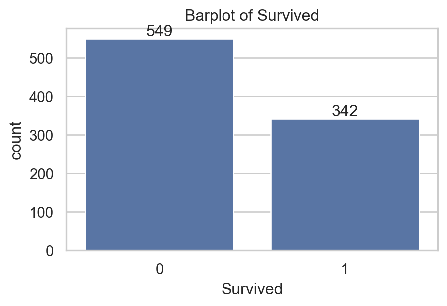
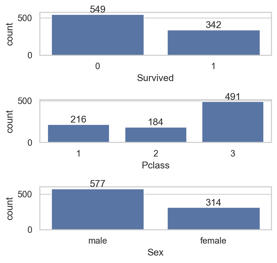
data[['Survived', 'Pclass', 'Age', 'Embarked']].head(5)                  # Show 5 first rows
Survived Pclass Age Embarked
0 0 3 22.0 S
1 1 1 38.0 C
2 1 3 26.0 S
3 1 1 35.0 S
4 0 3 35.0 S
  • Column Embarked is clearly different:
    • Performing \(+\), \(-\), \(\times\), \(\div\)… doesn’t make any sense!
    • Comparing \(<\), \(>\)… doesn’t make sense either!
  • Embarked is a Qualitative or Categorical data.
  • Age on the other hand is numbered:
    • Age \(50\) is older than \(30\).
    • Age \(20\) is \(5\) years younger than \(25\) or \(25-20=5\).
  • Age is a Quantitative or Numerical data.
  • Q1: How about other two columns?

Data Types

Quantity vs Quality

Data Types

Challenge

Code
data[['Sex', 'SibSp', 'Parch', 'Fare']].head()
Sex SibSp Parch Fare
0 male 1 0 7.2500
1 female 1 0 71.2833
2 female 0 0 7.9250
3 female 1 0 53.1000
4 male 0 0 8.0500


  • Q2: Define type of these columns.
Quantitative Qualitative
Column Dis Cont Nomi Ordi
Sex
SibSp
Parch
Fare
Quantitative Qualitative
Column Dis Cont Nomi Ordi
Sex
SibSp
Parch
Fare
Quantitative Qualitative
Column Dis Cont Nomi Ordi
Sex
SibSp
Parch
Fare
Quantitative Qualitative
Column Dis Cont Nomi Ordi
Sex
SibSp
Parch
Fare
Quantitative Qualitative
Column Dis Cont Nomi Ordi
Sex
SibSp
Parch
Fare


  • Now, let’s take a closer look!

Qualitative Data

Qualitative Data

Statistical values

data[['Pclass', 'Survived', 'Embarked', 'Sex']].head()
Pclass Survived Embarked Sex
0 3 0 S male
1 1 1 C female
2 3 1 S female
3 1 1 S female
4 3 0 S male
  • What values should we use to describe qualitative data?

  • Absolute Frequency: Number of accurences of category.

  • Relative Frequency: proportion/percentage of each category.

  • Mode: Category with highest frequency.

  • Example:
Code
freq_tab = data[['Pclass']].value_counts().to_frame()
freq_tab['proportion'] = data[['Pclass']].value_counts(normalize=True).round(2)
freq_tab.T
Pclass 3 1 2
count 491.00 216.00 184.00
proportion 0.55 0.24 0.21

Code
freq_tab = data[['Sex']].value_counts().to_frame()
freq_tab['proportion'] = data[['Sex']].value_counts(normalize=True).round(2)
freq_tab.T
Sex male female
count 577.00 314.00
proportion 0.65 0.35
  • Q3: I dare you to take care of the other two columns 😏!

Qualitative Data

Visualization

data[['Pclass', 'Survived', 'Embarked', 'Sex']].head()
Pclass Survived Embarked Sex
0 3 0 S male
1 1 1 C female
2 3 1 S female
3 1 1 S female
4 3 0 S male
  • What graph should we use to present qualitative data?
  • Countplot/Barplot: Represent each count/proportion by a bar.
  • Example:
import matplotlib.pyplot as plt
import seaborn as sns  # For graph
sns.set(style="whitegrid") # set nice background
plt.figure(figsize=(5,3))
ax = sns.countplot(data, x="Survived") # create graph
ax.set_title("Barplot of Survived") # add title
ax.bar_label(ax.containers[0]) # add number to bars
plt.show() # Show graph

Qualitative Data

Visualization

data[['Pclass', 'Survived', 'Embarked', 'Sex']].head()
Pclass Survived Embarked Sex
0 3 0 S male
1 1 1 C female
2 3 1 S female
3 1 1 S female
4 3 0 S male
  • What graph should we use to present qualitative data?
  • Countplot/Barplot: Represent each count/proportion by a bar.
  • Example:
import matplotlib.pyplot as plt
import seaborn as sns  # For graph
sns.set(style="whitegrid") # set nice background
plt.figure(figsize=(5,3))
ax = sns.countplot(data,x="Survived", stat="proportion")
ax.set_title("Barplot of Survived") # add title
ax.bar_label(ax.containers[0], fmt="%0.2f") # number
plt.show() # Show graph

Qualitative Data

Visualization

data[['Pclass', 'Survived', 'Embarked', 'Sex']].head()
Pclass Survived Embarked Sex
0 3 0 S male
1 1 1 C female
2 3 1 S female
3 1 1 S female
4 3 0 S male
  • What graph should we use to present qualitative data?
  • Pie chart: Represent count/proportion by circular slices.
  • Example:
import matplotlib.pyplot as plt
import seaborn as sns  # For graph
sns.set(style="whitegrid") # set nice background
plt.figure(figsize=(6,4))
tab = data['Embarked'].value_counts() # Compute 
plt.pie(tab, labels=tab.index, autopct='%0.2f%%') # graph
plt.title("Barplot of Pclass") # add title
plt.show() # Show graph

Qualitative Data

Visualization

data[['Pclass', 'Survived', 'Embarked', 'Sex']].head()
Pclass Survived Embarked Sex
0 3 0 S male
1 1 1 C female
2 3 1 S female
3 1 1 S female
4 3 0 S male
  • What graph should we use to present qualitative data?
  • Pie chart: Represent count/proportion by circular slices.

⚠️ Pie charts can be challenging to read with numerous categories. They’re harder to percieve when many categories have similar proportions.

  • Example:
import matplotlib.pyplot as plt
import seaborn as sns  # For graph
sns.set(style="whitegrid") # set nice background
plt.figure(figsize=(6,4))
tab = data['Embarked'].value_counts() # Compute 
plt.pie(tab, labels=tab.index, autopct='%0.2f%%') # graph
plt.title("Barplot of Pclass") # add title
plt.show() # Show graph

Qualitative Data

Summary

Quantitative Data

Quantitative Data

Statistical values

data[['Age', 'Fare', 'SibSp', 'Parch']].head()
Age Fare SibSp Parch
0 22.0 7.2500 1 0
1 38.0 71.2833 1 0
2 26.0 7.9250 0 0
3 35.0 53.1000 1 0
4 35.0 8.0500 0 0
  • What values should we use to describe quantitative data?
  • Quantiles: For data sorted in ascending order, the cut points divide the range into contiguous proportion intervals.

Examples:

  • Percentiles: Divides data into 100 equal parts.
  • Quartiles: The 25th (Q1), 50th (Q2 or median), and 75th (Q3) percentiles.

min 25% 50% 75% max
Fare 0.00 7.91 14.45 31.0 512.33
Age 0.42 20.12 28.00 38.0 80.00

Quantitative Data

Statistical values

data[['Age', 'Fare', 'SibSp', 'Parch']].head()
Age Fare SibSp Parch
0 22.0 7.2500 1 0
1 38.0 71.2833 1 0
2 26.0 7.9250 0 0
3 35.0 53.1000 1 0
4 35.0 8.0500 0 0
  • What values should we use to describe quantitative data?
  • Quantiles: For data sorted in ascending order, the cut points divide the range into contiguous proportion intervals.

Method to find Quartiles:

  • Sort the data in ascening order: \(X_1,...,X_n\).
  • If \(n\) is even: \(Q_2=\frac{X_{(n/2)}+X_{(n/2)+1}}{2}\).
    • \(Q_1\) is the middle point of the lower half data.
    • \(Q_3\) is the middle point of the upper half data.
  • If \(n\) is odd: \(Q_2=X_{(n+1)/2}\).
    • \(Q_1\) and \(Q_3\) can be computed as in the previous case.

Quantitative Data

Statistical values

data[['Age', 'Fare', 'SibSp', 'Parch']].head()
Age Fare SibSp Parch
0 22.0 7.2500 1 0
1 38.0 71.2833 1 0
2 26.0 7.9250 0 0
3 35.0 53.1000 1 0
4 35.0 8.0500 0 0
  • Median (Q2) is a value that describe Measure of Central Tendency.

  • Mean: Average value of all data points:

\[\color{blue}{\overline{X}=\frac{1}{n}\sum_{i=1}^nX_i=\frac{X_1+\dots+X_n}{n}}.\]

Examples:

mean = data[['Age','Fare']].mean()\
                        .to_frame()
mean.columns = ['Mean']
mean.T
Age Fare
Mean 29.699118 32.204208
  • The average age of passengers was around \(30\) years old.

  • In average, passengers spent approximately \(£32\) in fare.

Quantitative Data

Statistical values

data[['Age', 'Fare', 'SibSp', 'Parch']].head()
Age Fare SibSp Parch
0 22.0 7.2500 1 0
1 38.0 71.2833 1 0
2 26.0 7.9250 0 0
3 35.0 53.1000 1 0
4 35.0 8.0500 0 0
  • Two main Measure of dispersion:

  • Sample variance: average squared distance of data points from the Mean.

\[\color{blue}{\widehat{\sigma}^2=\frac{1}{n-1}\sum_{i=1}^n(X_i-\overline{X})^2}.\]

Examples:

var = data[['Age','Fare']].var()\
                        .to_frame()\
                        .round(3)
var.columns = ['Var']
var.T
Age Fare
Var 211.019 2469.437
  • Large variance means that data points are widely spread out from the Mean.

Quantitative Data

Statistical values

data[['Age', 'Fare', 'SibSp', 'Parch']].head()
Age Fare SibSp Parch
0 22.0 7.2500 1 0
1 38.0 71.2833 1 0
2 26.0 7.9250 0 0
3 35.0 53.1000 1 0
4 35.0 8.0500 0 0
  • Two main Measure of dispersion:

  • Sample standard deviation: Just the square root of Variance.

\[\color{blue}{\widehat{\sigma}=\sqrt{\widehat{\sigma}^2}=\sqrt{\frac{1}{n-1}\sum_{i=1}^n(X_i-\overline{X})^2}}.\]

Examples:

std = data[['Age','Fare']]\
        .apply(['var', 'std'])
std
Age Fare
var 211.019125 2469.436846
std 14.526497 49.693429
  • Large standard deviation (Std) means data points are spread out widely from the Mean.
  • Std has the same unit as \(X_i\).

Quantitative Data

Statistical Summary

data[['Age', 'Fare', 'SibSp', 'Parch']].head()
Age Fare SibSp Parch
0 22.0 7.2500 1 0
1 38.0 71.2833 1 0
2 26.0 7.9250 0 0
3 35.0 53.1000 1 0
4 35.0 8.0500 0 0
  • Statistical summary uses all key values to help us understand how the data is distributed:
    • Where the data is concentrated (mean/median).
    • How spread out it is (var/std)…

Examples:

data[['Age','Fare']]\
        .describe()  # for summary
Age Fare
count 714.000000 891.000000
mean 29.699118 32.204208
std 14.526497 49.693429
min 0.420000 0.000000
25% 20.125000 7.910400
50% 28.000000 14.454200
75% 38.000000 31.000000
max 80.000000 512.329200

Quantitative Data

Visualization: Boxplot

Age Fare SibSp Parch
0 22.0 7.2500 1 0
1 38.0 71.2833 1 0
2 26.0 7.9250 0 0
3 35.0 53.1000 1 0
4 35.0 8.0500 0 0
Code
import plotly.express as px
fig = px.box(data, x="Fare")
fig.update_layout(height=220,
                  width=500,
                  title="Boxplot of Fare")
fig.show()
  • Boxplots describe data using Quartiles and the range where data normally fall within.
  • Lower and upper fence are \(Q_1\) and \(Q_3\). Median \(Q_2\) is the middle line.
  • Interquartile range: \(\text{IQR}=Q_3-Q_1\), it’s the gap that covers central range of \(50\%\) of data.
  • Range: \([Q_1-1.5\text{IQR},Q_3+1.5\text{IQR}]\). If the data are normally distributed.
  • Data points that fall outside this range, can be considered Outliers (data that deviate away from usual observations).

Quantitative Data

Visualization: Boxplot

Code
import plotly.express as px
fig = px.box(data, x="Fare")
fig.update_layout(height=220,
                  width=500,
                  title="Boxplot of Fare")
fig.show()
  • This boxplot tells us that:
    • Fares range from \(£0\) to maximum fare of \(£512.33\).
    • \(Q_1=£7.9\) indicating that around \(25\%\) of passengers spent less than \(£7.9\) to get to the ship.
    • \(Q_2=£14.45\) (Median): \(\approx 50\%\) spent less than \(£14.45\).
    • \(Q_3=£31\): \(\approx 75\%\) spent less than \(£31\).
    • There are many outliers, passengers who spent more than upper fence of \(£65\), with largest fare of \(£512.33\).
  • Boxplots describe data using Quartiles and the range where data normally fall within.
  • Lower and upper fence are \(Q_1\) and \(Q_3\). Median \(Q_2\) is the middle line.
  • Interquartile range: \(\text{IQR}=Q_3-Q_1\), it’s the gap that covers central range of \(50\%\) of data.
  • Range: \([Q_1-1.5\text{IQR},Q_3+1.5\text{IQR}]\). If the data are normally distributed.
  • Data points that fall outside this range, can be considered Outliers (data that deviate away from usual observations).

Quantitative Data

Visualization: Histogram

Code
import plotly.express as px
fig = px.histogram(data, x="Age")
fig.update_layout(height=220, 
                  width=500,
                  title="Histogram of Age")
fig.show()
  • A histogram is constructed by:
    • Defining a grid range of bins: \(B_1, \dots, B_N\).
    • The height of each bar represents the count of \(X_i\) values that fall within the corresponding bin.
  • It describes the frequency of observations within each bin range.

Mathematical definition of histogram

  • Define bins: \(B_1,\dots, B_N\).
  • For any \(x\) and \(x\in B_k\) for some \(k\) then

\[\text{hist}(x)=\sum_{i=1}^n\mathbb{1}_{\{X_i\in B_k\}}.\]


For this example of Age:

  • Most passengers were between 16 and 52 years old.
  • There were more children younger than 10 years old than those around 10 years old.
  • There were fewer than 10 individuals in each age group older than 52 years old.

Quantitative Data

Visualization: Kernel Density Plot (KDE)

Code
import plotly.figure_factory as ff
age = [data[['Age']].dropna().values.reshape(-1)]
group_labels = ['distplot']
fig = ff.create_distplot(age, group_labels=group_labels, bin_size=1.9)
fig.update_layout(height=220,
                  width=500,
                  title="Histogram of Age")
fig.show()
  • A Kernel Density Plot is a smooth, continuous version of a histogram.
  • It describes the relative frequency of observations over ranges of values.
  • It has nicer mathematical properties than histograms.

Mathematical definition of KDE

  • If \(K\) is a smooth kernel function, for example: \(K(x)=e^{-x^2/2}\).
  • For a given \(h>0\) and for any \(x\):

\[\text{kde}(x)=\frac{1}{nh}\sum_{i=1}^nK\Big(\frac{x-X_i}{h}\Big).\]


  • Kernel density plot conveys similar information as histograms.
  • It’s often discussed in pobability and statistics classes.

Quantitative Data

Summary

Real examples

Real examples

Our Titanic Dataset

Qualitative columns

Code
qual_var = ['Survived', 'Pclass', 'Sex']
fig, axs = plt.subplots(3, 1, figsize=(5,4.75))
for i, va in enumerate(qual_var):
    sns.countplot(data[qual_var], x=va, ax=axs[i])
    axs[i].bar_label(axs[i].containers[0])
plt.tight_layout()
plt.show()

Quantitative columns

Code
quan_var = ['Age', 'SibSp', 'Parch', 'Fare']
fig, axs = plt.subplots(2, 2, figsize=(5,4.75))
for i, va in enumerate(quan_var):
    sns.histplot(data[quan_var], x=va, ax=axs[i//2, i%2], kde=True)
    if va == 'Fare':
        axs[i//2, i%2].set_xscale('log')
plt.tight_layout()
plt.show()

2. Data Visualization

Motivation

Motivation

Gapminder dataset (1704, 5)

  • This dataset captures the world’s evolution from \(1952\) to \(2007\).
  • Now, take a look at the data from year \(2007\).
Code
from gapminder import gapminder
data2007 = gapminder[gapminder.year == 2007]  # filter to year 2007
data2007.iloc[:5,:].drop(columns=['year']).style.hide()
country continent lifeExp pop gdpPercap
Afghanistan Asia 43.828000 31889923 974.580338
Albania Europe 76.423000 3600523 5937.029526
Algeria Africa 72.301000 33333216 6223.367465
Angola Africa 42.731000 12420476 4797.231267
Argentina Americas 75.320000 40301927 12779.379640

Motivation

Gapminder dataset (1704, 5)

  • This dataset captures the world’s evolution from \(1952\) to \(2007\).
  • Now, take a look at the data from year \(2007\) (summary).
Code
quan_vars = ["pop", "lifeExp", "gdpPercap"]
data2007[quan_vars].describe().transpose().drop(columns=["count", "25%", "75%"]).transpose()
pop lifeExp gdpPercap
mean 4.402122e+07 67.007423 11680.071820
std 1.476214e+08 12.073021 12859.937337
min 1.995790e+05 39.613000 277.551859
50% 1.051753e+07 71.935500 6124.371108
max 1.318683e+09 82.603000 49357.190170

Motivation

Gapminder dataset (1704, 5)

  • This dataset captures the world’s evolution from \(1952\) to \(2007\).
  • Now, take a look at the data from year \(2007\) (visualization).
Code
from plotly.subplots import make_subplots
import plotly.graph_objects as go
fig = make_subplots(rows=1, cols=3, 
              subplot_titles=("Boxplot of pop", "Violinplot of lifeExp", "Histogram of GDP Per Capita"))
fig.add_trace(go.Box(y=data2007['pop'], name="pop"), col=1, row=1)
fig.add_trace(go.Violin(y=data2007['lifeExp'], name="lifeExp"), row=1, col=2)
fig.add_trace(go.Histogram(x=data2007['gdpPercap'],
              name="gdpPercap"), row=1, col=3)
fig.update_layout(height=280, width=1000)
fig.update_yaxes(type="log", row=1, col=1)
fig.update_xaxes(title="Population", row=1, col=1)
fig.update_xaxes(title="Life Expectancy", row=1, col=2)
fig.update_xaxes(title="GDP Per Capita", row=1, col=3)
fig.show()

Bivariate Visualization

Bivariate Visualization

Quantitative vs quantitative: Scatterplot

  • Scatterplot shows trends/relation of quantitative pairs.
  • Let’s visualize relation: gdpPercap wih lifeExp & pop.
Code
import plotly.graph_objects as go
import plotly.express as px
data2007 = gapminder.query("year == 2007")
fig1 = px.scatter(data2007, x="gdpPercap", y="lifeExp", hover_name="country", opacity=0.7)
fig1.update_traces(marker=dict(size=10))
fig1.update_layout(height=350, width=500, title="The world GDP vs LifeExp in 2007")
fig1.show()
Code
data2007 = gapminder.query("year == 2007")
fig2 = px.scatter(data2007, x="gdpPercap", y="pop", hover_name="country", opacity=0.7)
fig2.update_traces(marker=dict(size=10))
fig2.update_layout(height=350, width=500, title="The world GDP vs Population in 2007")
fig2.show()

Bivariate Visualization

Quantitative vs quantitative: Scatterplot

  • Scatterplot shows trends/relation of the quantitative pair.
  • Let’s visualize relation: gdpPercap wih lifeExp & pop.
Code
fig1.update_layout(title="The world (log) GDP vs Population 2007 ")
fig1.update_xaxes(type="log")
fig1.show()
Code
fig2.update_layout(title="The world GDP vs (log) Population 2007 ")
fig2.update_yaxes(type="log")
fig2.show()

Bivariate Visualization

Quantitative vs quantitative: Scatterplot

  • GPD vs Life Expectancy:
    • General trend: Countries with high GPD tend to be healthier.
    • There are also a few countries with economy well above average yet health condition is still bad.


  • GPD vs Population:
    • General trend: no clear trend!
    • GDP per capita does not appear to be significantly influenced by a country’s population size.

Bivariate Visualization

Quantitative vs qualitative: Conditional

  • To see relation between Values within different Group, we can use:
    • Conditional Boxplots: boxplots within different groups.
    • Conditional Histogram/Density.
Code
sorted_data = data2007.sort_values(by='lifeExp')
fig = px.box(data2007, x="continent", y="lifeExp", hover_name="country", color="continent", category_orders={'continent': sorted_data['continent']})
fig.update_layout(title="Life Expectancy on each continent in 2007", height=300, width=450)
fig.show()
  • Key: The distinction of quantitative values between different groups indicates a connection between the pairs.

  • Example:

    • Clear distinction of lifeExp accross different continent suggests that there is a relation between the two.
    • continent is useful for predicting / explaining lifeExp.

Bivariate Visualization

Quantitative vs qualitative: Conditional

  • To see relation between Values within different Group, we can use:
    • Conditional Boxplots: boxplots within different groups.
    • Conditional Histogram/Density.
Code
import plotly.figure_factory as ff
group_labels = list(data2007.continent.unique())
hist_data = [data2007.lifeExp[data2007.continent == x] for x in group_labels]
colors = ["#f1ab17", "#f13c26", "#9be155", "#4ab8dc", "#d567f3"]
fig = ff.create_distplot(hist_data, group_labels, colors=colors,
                         bin_size=1.5, show_rug=False)
fig.update_layout(title="Life Expectancy on each continent in 2007", height=300, width=450)
fig.show()
  • Key: The distinction of quantitative values between different groups indicates a connection between the pairs.

  • Example:

    • Clear distinction of lifeExp accross different continent suggests that there is a relation between the two.
    • continent is useful for predicting / explaining lifeExp.

Bivariate Visualization

Quantitative vs qualitative: Conditional

  • How about GDP on each continent?
Code
sorted_data = data2007.sort_values(by='gdpPercap')
hist_data_gdp = [data2007.gdpPercap[data2007.continent == x] for x in group_labels]
colors = ["#f1ab17", "#f13c26", "#9be155", "#4ab8dc", "#d567f3"]
fig3 = px.box(data2007, x="continent", y="gdpPercap", hover_name="country", color="continent", category_orders={'continent': sorted_data['continent']})
fig3.update_layout(title="GDP per Capita on each continent in 2007", height=350, width=500)
fig3.show()
Code
sorted_data = data2007.sort_values(by='gdpPercap')
hist_data_gdp = [data2007.gdpPercap[data2007.continent == x] for x in group_labels]
colors = ["#f1ab17", "#f13c26", "#9be155", "#4ab8dc", "#d567f3"]
fig3 = px.violin(data2007, x="continent", y="gdpPercap", hover_name="country", color="continent", category_orders={'continent': sorted_data['continent']})
fig3.update_layout(title="GDP per Capita on each continent in 2007", height=350, width=500)
fig3.show()
  • Example:
    • The separation of GDP per Capita between coninents is not as clear as Life Expectancy, yet one can still see the differences.
    • continent is useful for predicting / explaining gdpPercap though not as strong/clear as with lifeExp.

Bivariate Visualization

Qualitative vs qualitative: mosaic plot

  • We don’t have many qualitative columns,
    I do grouped GDP:
    • If GDP \(\leq 33.33\%\) 👉 Developing
    • elif GDP \(\leq 66.66\%\) 👉 Emerging
    • else GDP \(\geq 66.66\%\) 👉 Developed.

Bivariate Visualization

Qualitative vs qualitative: mosaic plot

  • We don’t have many qualitative columns,
    I do grouped GDP:
    • If GDP \(\leq 33.33\%\) 👉 Developing
    • elif GDP \(\leq 66.66\%\) 👉 Emerging
    • else GDP \(\geq 66.66\%\) 👉 Developed.
  • Example:
    • As GDP seems to be related to continent, it remains true with categorical GDP.
    • In Asia, the three types of economic conditions are well balanced, whereas the majority of African countries are developing, followed by emerging economies.
Code
from statsmodels.graphics.mosaicplot import mosaic
import matplotlib.pyplot as plt
import pandas as pd
fig, ax = plt.subplots(figsize=(7, 5))
plt.rcParams.update({'font.size': 15})
def prop(key):
    if "Asia" in key:
        return {'color': '#51cb4b'}
    if "Africa" in key:
        return {'color': '#e35441'}
    if "Americas" in key:
        return {'color': '#41b4e3'}
    if "Europe" in key:
        return {'color': '#dda63e'}
    if "Oceania" in key:
        return {'color': '#b374df'}

data2007['gdp_category'] = pd.qcut(data2007['gdpPercap'], q=3, labels=['Developing', 'Emerging', 'Developed'])
mosaic(data2007.sort_values('continent'), ['continent','gdp_category'], 
    gap=0.01, properties = prop, 
    label_rotation=30, ax=ax)
plt.title("Mosaicplot of categorical GDP vs Continent")
plt.show()

Bivariate Visualization

Qualitative vs qualitative: grouped barplots

  • We don’t have many qualitative columns,
    I do grouped GDP:
    • If GDP \(\leq 33.33\%\) 👉 Developing
    • elif GDP \(\leq 66.66\%\) 👉 Emerging
    • else GDP \(\geq 66.66\%\) 👉 Developed.
  • Example:
    • As GDP seems to be related to continent, it remains true with categorical GDP.
    • In Asia, the three types of economic conditions are well balanced, whereas the majority of African countries are developing, followed by emerging economies.
Code
fig = px.histogram(
    data2007, x="continent", color="gdp_category")
fig.update_layout(width=510, height=470, 
    title='Stacked Barplot of Categorical GDP vs Continent')
fig.show()
Code
fig = px.histogram(
    data2007, x="continent", color="gdp_category", barmode='group')
fig.update_layout(width=510, height=470, title='Grouped Barplot of Categorical GDP vs Continent')
fig.show()

Multiple Information

Multiple Information

Color: quantitative & qualitative

  • Color can represent:
    • qualitative data (discrete color).
    • quantitative (in form of gradient)
Code
import numpy as np
data2007[' '] = np.repeat('Data', data2007.shape[0])
fig = px.scatter(
    data2007, x="gdpPercap", y="lifeExp",
    hover_name="country", size_max=80, color=" ")
fig.update_layout(width=472, height=400, title='Life Expectancy vs GDP per Capita & Continent')
fig.update_xaxes(type="log")
fig.show()

Multiple Information

Color: quantitative & qualitative

  • Color can represent:
    • qualitative data (discrete color).
    • quantitative (in form of gradient)
  • Example:
    • Color = continent, which is a categorical column.
Code
fig = px.scatter(
    data2007, x="gdpPercap", y="lifeExp", color="continent", hover_name="country", size_max=80)
fig.update_layout(width=500, height=400, title='Life Expectancy vs GDP per Capita & Continent')
fig.update_xaxes(type="log")
fig.show()

Multiple Information

Color: quantitative & qualitative

  • Color can represent:
    • qualitative data (discrete color).
    • quantitative (in form of gradient)
  • Example:
    • Color = continent, which is a categorical column.
    • Color = leftExp, which is a quantitative column.
Code
fig = px.scatter(
    data2007, x="gdpPercap", y="lifeExp", color="lifeExp", hover_name="country", size_max=80)
fig.update_layout(width=500, height=240, title='Life Expectancy vs GDP per Capita & Continent')
fig.update_xaxes(type="log")
fig.show()

Multiple Information

Shape/Symbol: qualitative

  • Shape for representing qualitative data.

  • Example:

    • Symbol = gdp_category.
    • Color = continent.

Combining numerous colors and symbols can complicate a graph.

Use them carefully and only when appropriate.

Code
fig = px.scatter(
    data2007, x="gdpPercap", y="lifeExp", color="continent", 
    hover_name="country", symbol='gdp_category', size_max=80)
fig.update_layout(width=500, height=350, title='Life Expectancy vs GDP per Capita & Continent')
fig.update_xaxes(type="log")
fig.show()

Multiple Information

Size: quantitative

  • Size for representing quantitative data.

  • Example:

    • Size = pop.
    • Color = continent.

Colors and size are common, and the resulting graphs are often called Bubble chart.

One shoule choose suitable max size to have a nice graph.

Code
fig = px.scatter(
    data2007, x="gdpPercap", y="lifeExp", color="continent",
    hover_name="country", size="pop", size_max=35)
fig.update_layout(width=500, height=370, title='Life Expectancy, GDP, Population & Continent')
fig.update_xaxes(type="log")
fig.show()

Multiple Information

3D: quantitative

  • All the previous options can be used with 3D scatter plot.

  • Example: Marketing

    • X = Youtube.
    • Y = Facebook.
    • Z = Sales.
    • Size = Newspaper.
    • Color = Newspaper.

Avoid 3D if they are not interactive [Section: “Don’t go 3D” by Claus O. Wilke (2019)].

Time series data

Time series data

Quantitative: lineplot

  • Let’s take a look at Oceania from 1952 to 2007.
Code
df_ocean = gapminder.query("continent == 'Oceania'")
fig = px.line(df_ocean, x='year', y='lifeExp',
    symbol="country", color="country",
    title="Evolution of Life Expectancy")
fig.update_layout(height=350, width=330)
fig.show()
Code
fig = px.line(df_ocean, x='year', y='pop',
    symbol="country", color="country",
    title="Evolution of Population")
fig.update_layout(height=350, width=330)
fig.show()
Code
fig = px.line(df_ocean, x='year', y='gdpPercap',
    symbol="country", color="country",
    title="Evolution of GDP per Capita")
fig.update_layout(height=350, width=330)
fig.show()
  • Is there any other country’s evolution you would like to see?

Time series data

Quantitative: lineplot

  • Is there any other country’s evolution you would like to see?

Time series data

Qualitative: Evoluational barplots

  • Let’s take a look at the evolution of GDP per capita categories for Asian countries over time.
Code
def cat_gdp(yearly_data):
    return pd.qcut(yearly_data, q=3, labels=['Developing', 'Emerging', 'Developed'])
df = gapminder
# Apply the function to each year
df['GDP_Category'] = df.groupby('year').apply(lambda x: cat_gdp(x.gdpPercap)).reset_index(level=0, drop=True)

df_Af = df.query("continent == 'Asia'")
# Aggregate the data
df_agg = df_Af.groupby(['year', 'GDP_Category']).size().reset_index(name='Count')

# Create the stacked bar chart
fig = px.bar(
    df_agg, x='year', y='Count', 
    color='GDP_Category', barmode='stack',
    title="Evolution of Asian Countries' GDP Categories from 1952 to 2007",
    labels={'Count': 'Number of Countries', 'year': 'Year'})

fig.update_layout(height=350, width=1000)
fig.show()

Animated Graphs

Animated Graphs

Animation with Plotly

Code
import plotly.express as px
df = px.data.gapminder()
fig_anime = px.scatter(df, x="gdpPercap", y="lifeExp", animation_frame="year", animation_group="country",
           size="pop", color="continent", hover_name="country",
           log_x=True, size_max=50, range_x=[100,100000], 
           range_y=[25,90])
fig_anime.update_layout(height=460, width=1000, 
    title="The Evolution of the World in a Single Graph")


“There is no such thing as information overload. There is only bad design.” – Edward Tufte.

🥳 Yeahhhh….


Let’s Party… 🥂