![]() Content
Content
 Content
Introduction & Brief History
World of Approximation
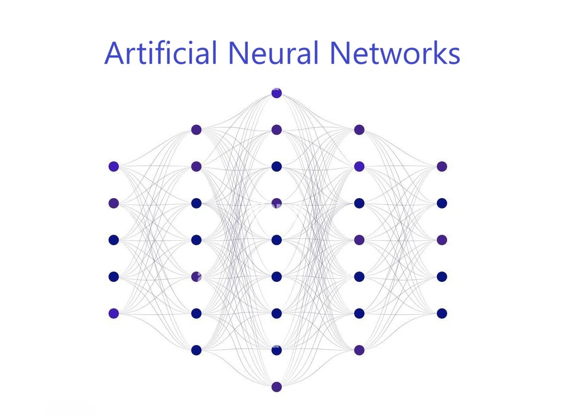
Neural Networks
Optimization
Applications
ITM-370: Data Analytics
![]()
Introduction & Brief History
World of Approximation
Neural Networks
Optimization
Applications
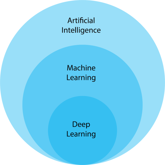
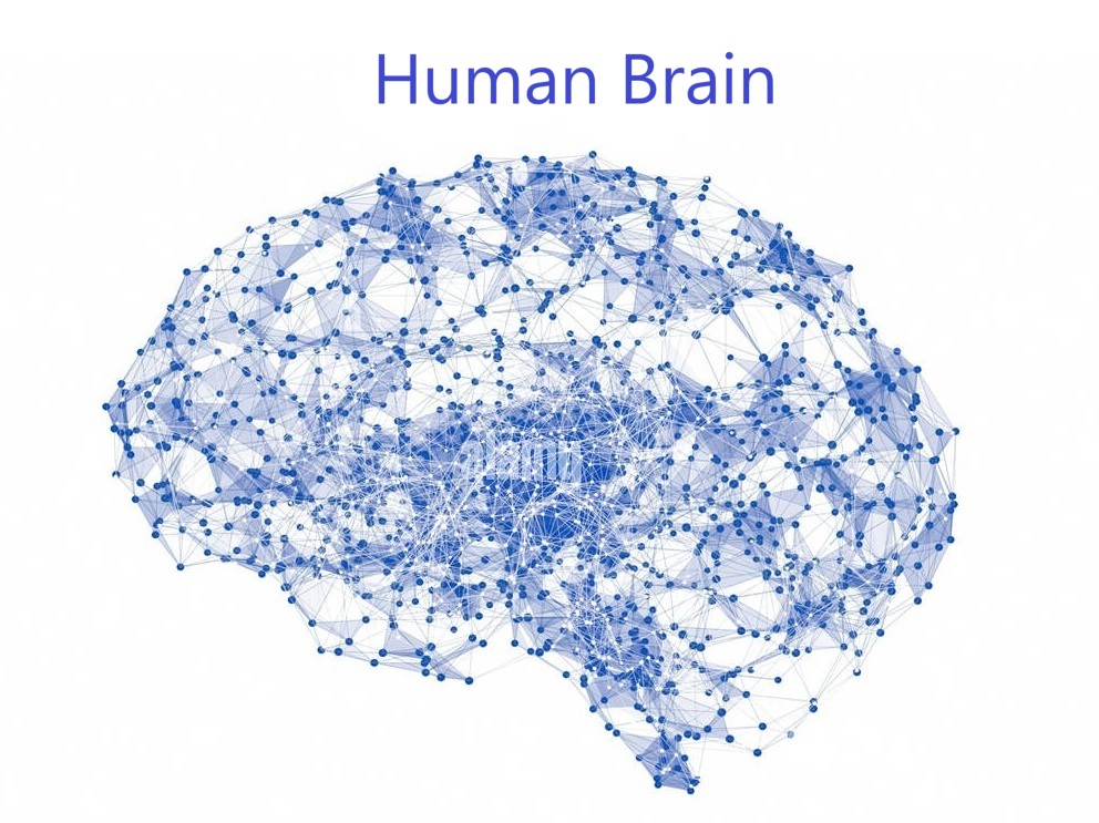
Deep Learning (DL) is a subset of Machine Learning (ML) that uses Multilayer Neural Networks, called Deep Neural Networks (DNN), to simulate the complex decision-making power of the human brain 🧠. Some form of deep learning powers most of the Artificial Intelligence (AI) applications in our lives today.


nonlinear activation function.
nonlinear activation function.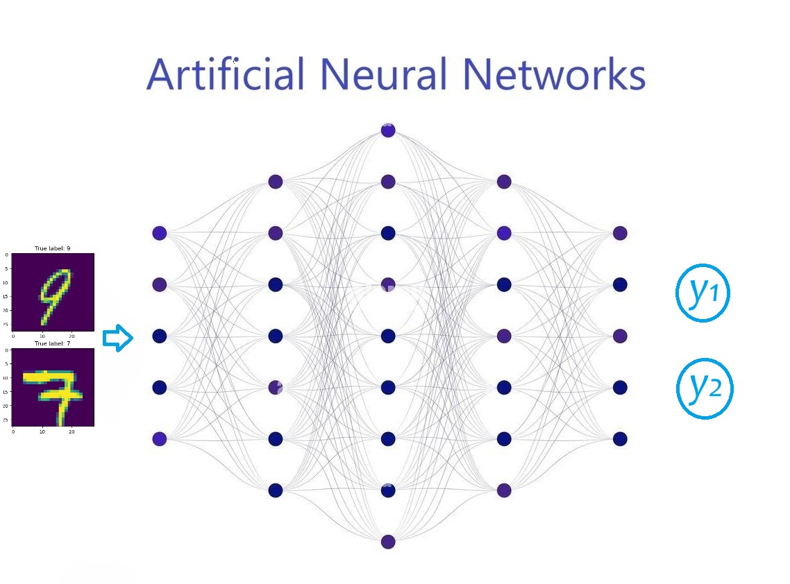
nonlinear activation function.

nonlinear activation function.
MLP using Keras.
Rings.![]()