Lab - Model Evaluation and Refinement

ITM-370: Data Analytics
Lecturer: HAS Sothea, PhD

Objective: Building a model is (SLR or MLR) is rather simple, but building a good model that can generalize well on unseen observations is more challenging. This practical lab aims at enhancing your practical skills in pushing the performance of your models on new unseen data using techniques introduced in the class.

The Jupyter Notebook for this Lab can be downloaded here: Lab_Model_Evaluation_Refinement.ipynb.

Or you can work with this notebook in Google Colab here: Lab_Model_Evaluation_Refinement.ipynb.

1. Importing `Abalone dataset`

You need internet to load the data by running the following codes. For more information about this data, read Abalone dataset.

# %pip install kagglehub   # if you have not installed "kagglehub" module yet
import kagglehub

# Download latest version
path = kagglehub.dataset_download("rodolfomendes/abalone-dataset")
print("Path to dataset files:", path)

# Import data
import pandas as pd
data = pd.read_csv(path + "/abalone.csv")
data.head()

Path to dataset files: C:\Users\hasso\.cache\kagglehub\datasets\rodolfomendes\abalone-dataset\versions\3

	Sex	Length	Diameter	Height	Whole weight	Shucked weight	Viscera weight	Shell weight	Rings
0	M	0.455	0.365	0.095	0.5140	0.2245	0.1010	0.150	15
1	M	0.350	0.265	0.090	0.2255	0.0995	0.0485	0.070	7
2	F	0.530	0.420	0.135	0.6770	0.2565	0.1415	0.210	9
3	M	0.440	0.365	0.125	0.5160	0.2155	0.1140	0.155	10
4	I	0.330	0.255	0.080	0.2050	0.0895	0.0395	0.055	7

A. What’s the dimension of this dataset? How many quantitative and qualitative variables are there in this dataset?

print(f'Dimension of the dataset: {data.shape}')
print(f'Quantitative variables: {list(data.columns[1:])}')
print(f'Quanlitative variables: {data.columns[0]}')

Dimension of the dataset: (4177, 9)
Quantitative variables: ['Length', 'Diameter', 'Height', 'Whole weight', 'Shucked weight', 'Viscera weight', 'Shell weight', 'Rings']
Quanlitative variables: Sex

B. Perform univariate analysis (compute statistical values and plot the distribution) on each variables of your dataset. The goal is to understand your data (the scale and how each column is distributed), detect missing values and outliers, etc.

Statistical values

data.iloc[:,1:].describe().drop(index=["count"])

	Length	Diameter	Height	Whole weight	Shucked weight	Viscera weight	Shell weight	Rings
mean	0.523992	0.407881	0.139516	0.828742	0.359367	0.180594	0.238831	9.933684
std	0.120093	0.099240	0.041827	0.490389	0.221963	0.109614	0.139203	3.224169
min	0.075000	0.055000	0.000000	0.002000	0.001000	0.000500	0.001500	1.000000
25%	0.450000	0.350000	0.115000	0.441500	0.186000	0.093500	0.130000	8.000000
50%	0.545000	0.425000	0.140000	0.799500	0.336000	0.171000	0.234000	9.000000
75%	0.615000	0.480000	0.165000	1.153000	0.502000	0.253000	0.329000	11.000000
max	0.815000	0.650000	1.130000	2.825500	1.488000	0.760000	1.005000	29.000000

data[["Sex"]].value_counts()

Sex
M      1528
I      1342
F      1307
Name: count, dtype: int64

There seems to be some Analone with $0.0$ height which are not reasonable. These are missing values and we should detect it.

n_missing = (data.Height == 0).sum()
print(f'The number of missing values: {n_missing}')

The number of missing values: 2

It’s just a very small proportion of the data, we don’t need waste time investigating its type missing type. We go ahead and drop these missing values.

data = data.loc[data.Height > 0,:]
data.describe()

	Length	Diameter	Height	Whole weight	Shucked weight	Viscera weight	Shell weight	Rings
count	4175.000000	4175.00000	4175.000000	4175.000000	4175.000000	4175.000000	4175.000000	4175.000000
mean	0.524065	0.40794	0.139583	0.829005	0.359476	0.180653	0.238834	9.935090
std	0.120069	0.09922	0.041725	0.490349	0.221954	0.109605	0.139212	3.224227
min	0.075000	0.05500	0.010000	0.002000	0.001000	0.000500	0.001500	1.000000
25%	0.450000	0.35000	0.115000	0.442250	0.186250	0.093500	0.130000	8.000000
50%	0.545000	0.42500	0.140000	0.800000	0.336000	0.171000	0.234000	9.000000
75%	0.615000	0.48000	0.165000	1.153500	0.502000	0.253000	0.328750	11.000000
max	0.815000	0.65000	1.130000	2.825500	1.488000	0.760000	1.005000	29.000000

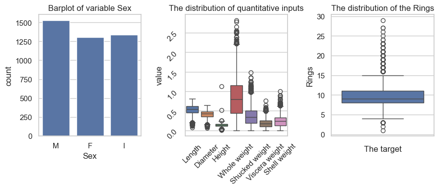
Visualize the distribution of the columns

quan_vars = data.columns[1:]
qual_var = "Sex"

import seaborn as sns
import matplotlib.pyplot as plt
sns.set(style="whitegrid")
_, ax = plt.subplots(1,3, figsize=(9, 4))

sns.countplot(data, x="Sex", ax=ax[0])
ax[0].set_title("Barplot of variable Sex")
ax[0].set_title

sns.boxplot(data[quan_vars[:-1]].melt(), x="variable", y="value", hue="variable", ax=ax[1])
ax[1].tick_params(labelrotation=45)
ax[1].set_title("The distribution of quantitative inputs")
ax[1].set_xlabel("")

sns.boxplot(data, y="Rings", ax=ax[2])
ax[2].set_title("The distribution of the Rings")
ax[2].set_xlabel("The target")
plt.tight_layout()
plt.show()

It looks like there are some outliers in both the target and inputs. We just notice this but proceed without removing them.

2. Correlation matrix, SLR and MLR

A. Compute the correlation matrix of this data using pd.corr() function. Describe what you observed from this correlation matrix.

data[quan_vars].corr().style.background_gradient()

	Length	Diameter	Height	Whole weight	Shucked weight	Viscera weight	Shell weight	Rings
Length	1.000000	0.986802	0.828108	0.925217	0.897859	0.902960	0.898419	0.556464
Diameter	0.986802	1.000000	0.834298	0.925414	0.893108	0.899672	0.906084	0.574418
Height	0.828108	0.834298	1.000000	0.819886	0.775621	0.798908	0.819596	0.557625
Whole weight	0.925217	0.925414	0.819886	1.000000	0.969389	0.966354	0.955924	0.540151
Shucked weight	0.897859	0.893108	0.775621	0.969389	1.000000	0.931924	0.883129	0.420597
Viscera weight	0.902960	0.899672	0.798908	0.966354	0.931924	1.000000	0.908186	0.503562
Shell weight	0.898419	0.906084	0.819596	0.955924	0.883129	0.908186	1.000000	0.627928
Rings	0.556464	0.574418	0.557625	0.540151	0.420597	0.503562	0.627928	1.000000

It appears that “Shell wieght” is the most correlated input to the target with the highest correlation around $0.63$ while other input-output correlations ranged from $0.42$ tà $0.56$, and Shucked Weight is the less informative one. Lastly, it’s worth noted that there are many highly correlated inputs in this dataset with the highest colinearity greater than $0.98£ between Diameter and Length.

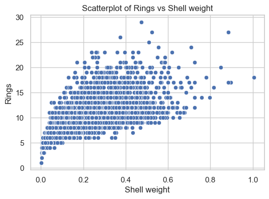
B. Draw the scatterplot of the target Rings vs the most correlated input.

plt.figure(figsize=(6, 4))
sns.scatterplot(data, x="Shell weight", y="Rings")
plt.title("Scatterplot of Rings vs Shell weight")
plt.show(block=False)

This scatterplot shows that Shell Weight seems to carry significant information about the Rings. Analone with heavier shell weights tend to have more rings.

Here, I split the data into two parts. You are allowed to use only the training part for building models. The testing part will be used to evaluate the models’ performance.

from sklearn.model_selection import train_test_split
X_train, X_test, y_train, y_test = train_test_split(
                                        data.iloc[:,1:8], 
                                        data['Rings'], 
                                        test_size=0.2, 
                                        random_state=42)

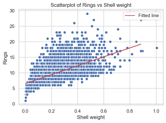
C. Fit a SLR model using the most correlated input to predict the Rings of abalone. - Draw the fitted line on the previous scatterplot. - Compute $R^2$ and explain the observed value. - Compute Mean Suared Error on the test data (Test MSE). - Analyze the residuals and conclude.

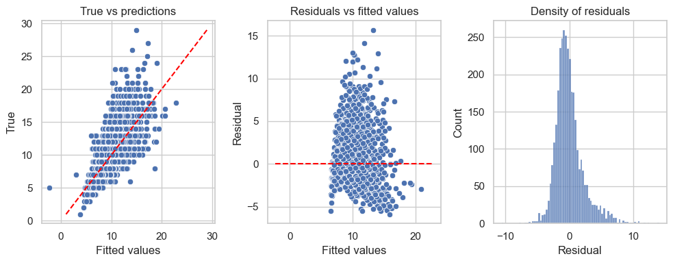
# Fit SLR model
from sklearn.linear_model import LinearRegression

# Build the SLR model
slr = LinearRegression().fit(X_train[['Shell weight']], y_train)
y_hat = slr.predict(X_test[["Shell weight"]])                   # make prediction on the test data

# Fit linear line to the scatterplot
plt.figure(figsize=(6, 4))
sns.scatterplot(data, x="Shell weight", y="Rings")
plt.plot(X_test['Shell weight'], y_hat, 'r', label="Fitted line")
plt.title("Scatterplot of Rings vs Shell weight")
plt.legend()
plt.show()

import numpy as np
from sklearn.metrics import r2_score, mean_squared_error
pred_train = slr.predict(X_train[['Shell weight']])
print(f'R-squared: {np.round(r2_score(y_train, pred_train),3)}')
print(f'Test MSE: {np.round(mean_squared_error(y_test, y_hat),3)}')

R-squared: 0.392
Test MSE: 6.841

R-squared indicates that around 40% variation of the target Rings can be captured or explained by the model. Now look at the residuals.

resid = pd.DataFrame({
    "True" : y_train,
    "Fitted values": pred_train,
    "Residual": y_train-pred_train}
)

_, ax = plt.subplots(1,3, figsize=(10, 4))
sns.scatterplot(resid, x="Fitted values", y="True", ax=ax[0])
sns.lineplot(x=[np.min(y_train), np.max(y_train)], y=[np.min(y_train), np.max(y_train)], ax=ax[0], color="red", linestyle="--")
ax[0].set_title("True vs predictions")

sns.scatterplot(resid, x="Fitted values", y="Residual", ax=ax[1])
sns.lineplot(x=[np.min(pred_train), np.max(pred_train)], y=[0, 0], ax=ax[1], color="red", linestyle="--")
ax[1].set_title("Residuals vs fitted values")

sns.histplot(resid, x="Residual", ax=ax[2])
ax[2].set_title("Density of residuals")
plt.tight_layout()
plt.show()

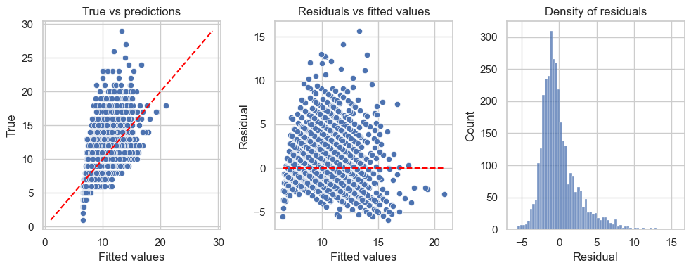
It’s clear that the model did not capture all the information from the target as the points in the first graph are not aligned closely to the red line $y=x$. The residuals are not symmetrically distributed around horizontal axis in the second graph, and the variance is not consistent either. The third graph tells us that the residuals seem not normally distributed.

D. Fit MLR using all inputs. Compute: - Compute $R^2$, adjusted $R_{\text{adj}}^2$ and explain the observed value. - Compute Mean Suared Error on the test data (Test MSE). - Analyze the residuals and conclude.

# Build the MLR model
mlr = LinearRegression().fit(X_train, y_train)
y_hat1 = mlr.predict(X_test)                   # make prediction on the test data

pred_train1 = mlr.predict(X_train)
n, d = X_train.shape
print(f'R-squared: {np.round(r2_score(y_train, pred_train1),3)}')
print(f'Adjusted R-squared: {np.round(1-(1-r2_score(y_train, pred_train1))*(n-1)/(n-d-1),3)}')
print(f'Test MSE: {np.round(mean_squared_error(y_test, y_hat1),3)}')

All_Test_MSE = {"SLR": mean_squared_error(y_test, y_hat1)}

R-squared: 0.518
Adjusted R-squared: 0.517
Test MSE: 5.049

This model seems to do a better job than SLR with R-squared around $0.5$ means that the model can capture around 52% of the variation of the target.

resid1 = pd.DataFrame({
    "True" : y_train,
    "Fitted values": pred_train1,
    "Residual": y_train-pred_train1}
)

_, ax = plt.subplots(1,3, figsize=(10, 4))
sns.scatterplot(resid1, x="Fitted values", y="True", ax=ax[0])
sns.lineplot(x=[np.min(y_train), np.max(y_train)], y=[np.min(y_train), np.max(y_train)], ax=ax[0], color="red", linestyle="--")
ax[0].set_title("True vs predictions")

sns.scatterplot(resid, x="Fitted values", y="Residual", ax=ax[1])
sns.lineplot(x=[np.min(pred_train1), np.max(pred_train1)], y=[0, 0], ax=ax[1], color="red", linestyle="--")
ax[1].set_title("Residuals vs fitted values")

sns.histplot(resid1, x="Residual", ax=ax[2])
ax[2].set_title("Density of residuals")
plt.tight_layout()
plt.show()

The residuals also seem to be better than the previous SLR model (the first graph) but there are still many pattern left in the residuals.

3. Polynomial Regression and Regularized Linear Models

A. Build polynomial regression with different degree $n\in\{2,3,...,10\}$ of the best correlated input to predict Rings. Compute Test MSE for each case.

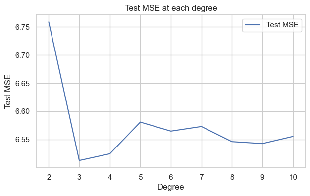
from sklearn.preprocessing import PolynomialFeatures
degrees = list(range(2,11))
mse = []
for deg in degrees:
    poly = PolynomialFeatures(degree=deg)
    X_poly = poly.fit_transform(X_train[['Shell weight']])
    model = LinearRegression().fit(X_poly, y_train)

    # MSE
    X_poly_test = poly.transform(X_test[['Shell weight']])
    mse.append(mean_squared_error(y_test, model.predict(X_poly_test)))
    All_Test_MSE['Poly. '+str(deg)] = mean_squared_error(y_test, model.predict(X_poly_test))

plt.figure(figsize=(7,4))
plt.plot(degrees, mse, label="Test MSE")
plt.title("Test MSE at each degree")
plt.xlabel("Degree")
plt.ylabel("Test MSE")
plt.legend()
plt.show()

This graph indicates that degree $3$ polynomial features of Shell weight appear to have the best performance in predicting the testing data, as evidenced by the lowest Test MSE. This suggests that a polynomial of degree $3$ may be a more effective model than a linear one. However, to ensure a comprehensive evaluation, we can perform cross-validation to assess the overall performance of polynomials with different degrees across various subsets of the training data

Perform $10$-fold Cross-validation to select the best degree $n$. Hint: see slide 20.

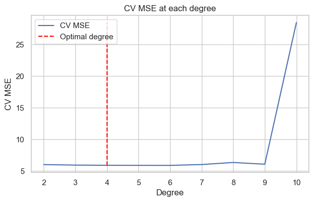
from sklearn.model_selection import cross_val_score
cv_mse = []
CV_ALL_MSE = {}
for deg in degrees:
    poly = PolynomialFeatures(degree=deg)
    X_poly = poly.fit_transform(X_train[['Shell weight']])
    model = LinearRegression()
    mse_ = -cross_val_score(model, X_poly, y_train, cv=10, scoring="neg_mean_squared_error").mean()
    CV_ALL_MSE['Poly. '+str(deg)] = mse_

    # MSE
    cv_mse.append(mse_)

opt_deg = np.argmin(cv_mse)
print(f'Optimal CV MSE: {np.min(np.round(cv_mse,3))} at optimal degree:{opt_deg}')
plt.figure(figsize=(7,4))
plt.plot(degrees, cv_mse, label="CV MSE")
plt.vlines(opt_deg, ymin=np.min(cv_mse), ymax=np.max(cv_mse), linestyles='--', colors='red', label="Optimal degree")
plt.title("CV MSE at each degree")
plt.xlabel("Degree")
plt.ylabel("CV MSE")
plt.legend()
plt.show()

Optimal CV MSE: 5.877 at optimal degree:4

This graph reveals that polynomial degree $4$ is slightly better than polynomial degree $3$ in predicting different subsets of the data via cross-validation splits. However, we should not feel that degree $4$ is really better than $2,3,5,6$ and $7$ because the differences in MSE are too insignificant.

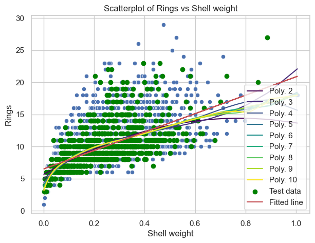
Let’s see how they fits to the data:

plt.figure(figsize=(7, 5))
sns.scatterplot(data, x="Shell weight", y="Rings")
colors = plt.cm.viridis(np.linspace(0, 1, len(degrees)))

# Fit degree 4 model
for deg, col in zip(degrees, colors):
    poly = PolynomialFeatures(degree=deg)
    X_poly = poly.fit_transform(X_train[['Shell weight']])
    ply = LinearRegression().fit(X_poly, y_train)
    y_poly_pred = ply.predict(X_poly)
    id_sort = np.argsort(X_train["Shell weight"])

    # Fit linear line to the scatterplot
    plt.plot(X_train[["Shell weight"]].values.reshape(-1)[id_sort], y_poly_pred[id_sort], label=f"Poly. {deg}", color=col)
plt.scatter(x=X_test['Shell weight'], y=y_test, c="green", label="Test data")
plt.plot(X_train['Shell weight'], pred_train, 'r', label="Fitted line")
plt.title("Scatterplot of Rings vs Shell weight")
plt.legend()
plt.show()

B. Perform $10$-fold Cross-validation to tune the best penalization strength $\alpha$ of Ridge regression model for predicting Rings. Hint: see slide 24. - We will build Ridge regression on full input data then compute Test MSE and compare it to the previous models.

from sklearn.linear_model import Ridge
# List of all degrees to search over
alphas = list(np.linspace(0.00001, 3, 50)) + list(np.linspace(3.1, 100, 50))
# List to store all losses
loss = []
test_mse = []
coefficients = {f'alpha={alpha}': [] for alpha in alphas}
for alp in alphas:
    model = Ridge(alpha=alp)
    mse = -cross_val_score(model, X_train, y_train, cv=10, 
                scoring='neg_mean_squared_error').mean()
    loss.append(mse)
    
    # Fit
    model.fit(X_train, y_train)
    coefficients[f'alpha={alp}'] = model.coef_
    test_mse.append(mean_squared_error(y_test, model.predict(X_test)))

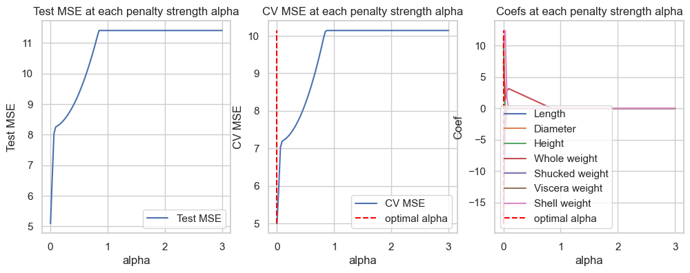
fig, axes = plt.subplots(1, 3, figsize=(12,4))
pd_coef = pd.DataFrame(coefficients, index=X_train.columns)
# Test error
axes[0].plot(alphas, test_mse, label="Test MSE")
axes[0].set_title("Test MSE at each penalty strength alpha")
axes[0].legend()
axes[0].set_xlabel("alpha")
axes[0].set_xscale('log')
axes[0].set_ylabel("Test MSE")

id_min = np.argmin(loss)
print(f'Optimal regularization strength alpha for Ridge regression: {alphas[id_min]}')
axes[1].plot(alphas, loss, label="CV MSE")
axes[1].vlines(x=alphas[id_min], ymin=np.min(loss), ymax=np.max(loss), label="optimal alpha", color="red", linestyle="--")
axes[1].set_title("CV MSE at each penalty strength alpha")
axes[1].legend()
axes[1].set_xscale('log')
axes[1].set_xlabel("alpha")
axes[1].set_ylabel("CV MSE")

axes[2].plot(alphas, pd_coef.transpose(), label=pd_coef.index)
axes[2].vlines(x=alphas[id_min], ymin=np.min(pd_coef), ymax=np.max(pd_coef), label="optimal alpha", color="red", linestyle="--")
axes[2].set_title("Coefs at each penalty strength alpha")
axes[2].legend()
axes[2].set_xscale('log')
axes[2].set_xlabel("alpha")
axes[2].set_ylabel("Coef")
plt.show()

Optimal regularization strength alpha for Ridge regression: 0.6734771428571428

The first graph is the performance of Ridge regression at each value of $\alpha$ on the testing data. On the other hand, the second graph illustrates the performance of Ridge regression on cross-validation subsets. The last graph shows the values of the coefficients of the model at each value of penalty parameter $\alpha$.

We can see that optimal strength $\alpha\approx 0.67$ by cross-validation method. The average CV MSE at this level of penalty strength is given below.

All_Test_MSE['Ridge'] = test_mse[id_min]
CV_ALL_MSE['Ridge'] = loss[id_min]
print(f"Cross-validation MSE: {loss[id_min]}")
print(f"Test MSE: {test_mse[id_min]}")

Cross-validation MSE: 4.953797459164008
Test MSE: 5.126732705305683

C. Perform $10$-fold Cross-validation to tune the best penalization strength $\alpha$ of Lasso regression model for predicting Rings. Hint: see slide 24. - Compute Test MSE and compare it to the previous models. - How many inputs are retained by Lasso?

from sklearn.linear_model import Lasso
# List of all degrees to search over
alphas = list(np.linspace(0.001, 3, 100))
# List to store all losses
loss = []
test_mse = []
coefficients = {f'alpha={alpha}': [] for alpha in alphas}
for alp in alphas:
    model = Lasso(alpha=alp)
    mse = -cross_val_score(model, X_train, y_train, cv=10, 
                scoring='neg_mean_squared_error').mean()
    loss.append(mse)

    # Fit
    model.fit(X_train, y_train)
    coefficients[f'alpha={alp}'] = model.coef_
    test_mse.append(mean_squared_error(y_test, model.predict(X_test)))

fig, axes = plt.subplots(1, 3, figsize=(12,4))
pd_coef = pd.DataFrame(coefficients, index=X_train.columns)
# Test error
axes[0].plot(alphas, test_mse, label="Test MSE")
axes[0].set_title("Test MSE at each penalty strength alpha")
axes[0].legend()
axes[0].set_xlabel("alpha")
# axes[0].set_xscale('log')
axes[0].set_ylabel("Test MSE")

id_min = np.argmin(loss)
print(f'Optimal regularization strength alpha for Lasso regression: {alphas[id_min]}')
axes[1].plot(alphas, loss, label="CV MSE")
axes[1].vlines(x=alphas[id_min], ymin=np.min(loss), ymax=np.max(loss), label="optimal alpha", color="red", linestyle="--")
axes[1].set_title("CV MSE at each penalty strength alpha")
axes[1].legend()
# axes[1].set_xscale('log')
axes[1].set_xlabel("alpha")
axes[1].set_ylabel("CV MSE")

axes[2].plot(alphas, pd_coef.transpose(), label=pd_coef.index)
axes[2].vlines(x=alphas[id_min], ymin=np.min(pd_coef), ymax=np.max(pd_coef), label="optimal alpha", color="red", linestyle="--")
axes[2].set_title("Coefs at each penalty strength alpha")
axes[2].legend()
# axes[2].set_xscale('log')
axes[2].set_xlabel("alpha")
axes[2].set_ylabel("Coef")
plt.show()

Optimal regularization strength alpha for Lasso regression: 0.001

All_Test_MSE['Lasso'] = test_mse[id_min]
CV_ALL_MSE['Lasso'] = loss[id_min]
print(f"Cross-validation MSE: {loss[id_min]}")
print(f"Test MSE: {test_mse[id_min]}")

Cross-validation MSE: 4.995800296285283
Test MSE: 5.088192636942236

Polynomial with Regularitation

Now we combine regularization with higher polynomial degree.

Ridge regression

from sklearn.linear_model import Ridge
# List of all degrees to search over
poly = PolynomialFeatures(degree=4)
X_poly = poly.fit_transform(X_train)
X_poly_test = poly.transform(X_test)

alphas = list(np.linspace(0.00001, 3, 50)) + list(np.linspace(3.1, 100, 50))
# List to store all losses
loss = []
test_mse = []
coefficients = {f'alpha={alpha}': [] for alpha in alphas}
for alp in alphas:
    model = Ridge(alpha=alp)
    mse = -cross_val_score(model, X_poly, y_train, cv=10, 
                scoring='neg_mean_squared_error').mean()
    loss.append(mse)

    # Fit
    model.fit(X_poly, y_train)
    coefficients[f'alpha={alp}'] = model.coef_
    test_mse.append(mean_squared_error(y_test, model.predict(X_poly_test)))

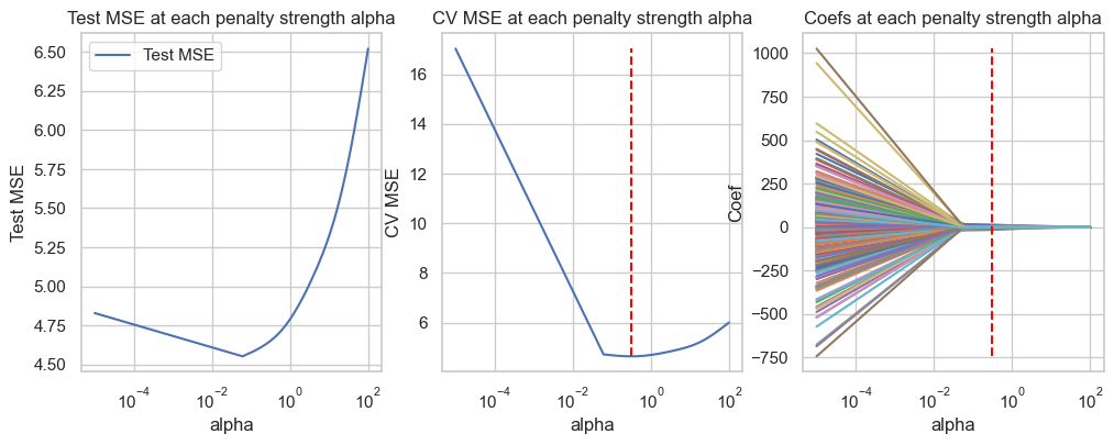
fig, axes = plt.subplots(1, 3, figsize=(12,4))
pd_coef = pd.DataFrame(coefficients, index=poly.get_feature_names_out(input_features=X_train.columns))
# Test error
axes[0].plot(alphas, test_mse, label="Test MSE")
axes[0].set_title("Test MSE at each penalty strength alpha")
axes[0].legend()
axes[0].set_xlabel("alpha")
axes[0].set_xscale('log')
axes[0].set_ylabel("Test MSE")

id_min = np.argmin(loss)
print(f'Optimal regularization strength alpha for Ridge regression: {alphas[id_min]}')
axes[1].plot(alphas, loss, label="CV MSE")
axes[1].vlines(x=alphas[id_min], ymin=np.min(loss), ymax=np.max(loss), label="optimal alpha", color="red", linestyle="--")
axes[1].set_title("CV MSE at each penalty strength alpha")
axes[1].set_xscale('log')
axes[1].set_xlabel("alpha")
axes[1].set_ylabel("CV MSE")

axes[2].plot(alphas, pd_coef.transpose(), label=pd_coef.index)
axes[2].vlines(x=alphas[id_min], ymin=np.min(pd_coef), ymax=np.max(pd_coef), label="optimal alpha", color="red", linestyle="--")
axes[2].set_title("Coefs at each penalty strength alpha")
axes[2].set_xscale('log')
axes[2].set_xlabel("alpha")
axes[2].set_ylabel("Coef")
plt.show()

Optimal regularization strength alpha for Ridge regression: 0.30613142857142855

All_Test_MSE['Poly-Ridge'] = test_mse[id_min]
CV_ALL_MSE['Poly-Ridge'] = loss[id_min]
print(f"Cross-validation MSE: {loss[id_min]}")
print(f"Test MSE: {test_mse[id_min]}")

Cross-validation MSE: 4.647400669206419
Test MSE: 4.647813719255127

Lasso regression

from sklearn.linear_model import Lasso
# List of all degrees to search over
alphas = list(np.linspace(0.00001, 10, 100))
# List to store all losses
loss = []
test_mse = []
coefficients = {f'alpha={alpha}': [] for alpha in alphas}
for alp in alphas:
    model = Lasso(alpha=alp)
    mse = -cross_val_score(model, X_poly, y_train, cv=10, 
                scoring='neg_mean_squared_error').mean()
    loss.append(mse)

    # Fit
    model.fit(X_poly, y_train)
    coefficients[f'alpha={alp}'] = model.coef_
    test_mse.append(mean_squared_error(y_test, model.predict(X_poly_test)))

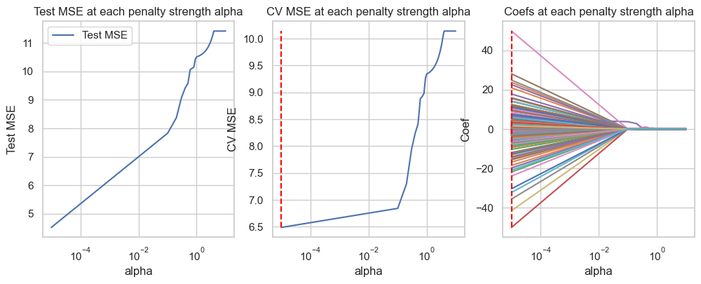
fig, axes = plt.subplots(1, 3, figsize=(12,4))
pd_coef = pd.DataFrame(coefficients, index=poly.get_feature_names_out(input_features=X_train.columns))
# Test error
axes[0].plot(alphas, test_mse, label="Test MSE")
axes[0].set_title("Test MSE at each penalty strength alpha")
axes[0].legend()
axes[0].set_xlabel("alpha")
axes[0].set_xscale('log')
axes[0].set_ylabel("Test MSE")

id_min = np.argmin(loss)
print(f'Optimal regularization strength alpha for Ridge regression: {alphas[id_min]}')
axes[1].plot(alphas, loss, label="CV MSE")
axes[1].vlines(x=alphas[id_min], ymin=np.min(loss), ymax=np.max(loss), label="optimal alpha", color="red", linestyle="--")
axes[1].set_title("CV MSE at each penalty strength alpha")
axes[1].set_xscale('log')
axes[1].set_xlabel("alpha")
axes[1].set_ylabel("CV MSE")

axes[2].plot(alphas, pd_coef.transpose(), label=pd_coef.index)
axes[2].vlines(x=alphas[id_min], ymin=np.min(pd_coef), ymax=np.max(pd_coef), label="optimal alpha", color="red", linestyle="--")
axes[2].set_title("Coefs at each penalty strength alpha")
axes[2].set_xscale('log')
axes[2].set_xlabel("alpha")
axes[2].set_ylabel("Coef")
plt.show()

Optimal regularization strength alpha for Ridge regression: 1e-05

All_Test_MSE['Poly-Lasso'] = test_mse[id_min]
CV_ALL_MSE['Poly-Lasso'] = loss[id_min]
print(f"Cross-validation MSE: {loss[id_min]}")
print(f"Test MSE: {test_mse[id_min]}")

Cross-validation MSE: 6.485597009720304
Test MSE: 4.520971235467517

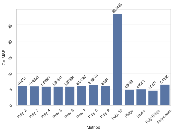
Conclusion

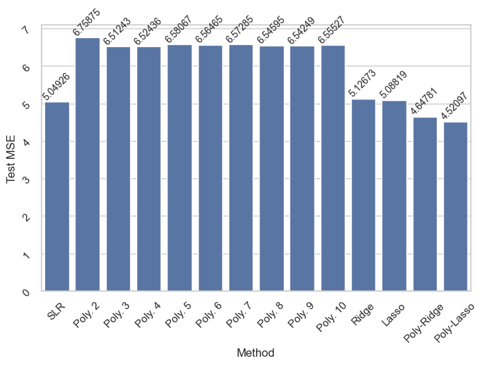
According to test MSE, polynomial features with Lasso constraint seems to perform better than other methods.
However, polynomial features with Ridge constraint seems to perform slightly better than the others in terms of Cross-validation MSE suggesting that it is more suitable in generalizing to new unseen observations.
We report the overall performances in the following tables.
Note that this analysis is done based on the whole data without taking in account the effect of outliers.
This dataset contains a lot of outliers and methods that takes into account clustering structure of the input might be suitable for such a dataset, for example, See KFC Procedure, Has et al. (2021).

print('Test MSE of all methods:')
df1 = pd.DataFrame(All_Test_MSE, index=['MSE'])
plt.figure(figsize=(8,5))
ax = sns.barplot(df1.melt(), x="variable", y="value")
ax.tick_params(labelrotation = 45)
ax.bar_label(ax.containers[0], fontsize=10, rotation=45)
ax.set_xlabel("Method")
ax.set_ylabel("Test MSE")
df1

Test MSE of all methods:

	SLR	Poly. 2	Poly. 3	Poly. 4	Poly. 5	Poly. 6	Poly. 7	Poly. 8	Poly. 9	Poly. 10	Ridge	Lasso	Poly-Ridge	Poly-Lasso
MSE	5.049255	6.758753	6.512433	6.524356	6.580672	6.56465	6.572854	6.545954	6.542486	6.555271	5.126733	5.088193	4.647814	4.520971

print("Corss validation of all methods:")
df2 = pd.DataFrame(CV_ALL_MSE, index=["MSE"])
plt.figure(figsize=(8,5))
ax = sns.barplot(df2.melt(), x="variable", y="value")
ax.tick_params(labelrotation = 45)
ax.bar_label(ax.containers[0], fontsize=10, rotation=45)
ax.set_xlabel("Method")
ax.set_ylabel("CV MSE")
df2

Corss validation of all methods:

	Poly. 2	Poly. 3	Poly. 4	Poly. 5	Poly. 6	Poly. 7	Poly. 8	Poly. 9	Poly. 10	Ridge	Lasso	Poly-Ridge	Poly-Lasso
MSE	6.005101	5.923215	5.893669	5.88341	5.876838	6.013628	6.338744	6.063998	28.442479	4.953797	4.9958	4.647401	6.485597

1. Importing Abalone dataset

2. Correlation matrix, SLR and MLR

3. Polynomial Regression and Regularized Linear Models

Polynomial with Regularitation

Conclusion

Further readings

1. Importing `Abalone dataset`