from keras.datasets import mnist

(X_train, label_train), (X_test, label_test) = mnist.load_data()

# Visualize

import matplotlib.pyplot as plt

plt.imshow(X_train[0,:,:])
plt.axis("off")
plt.show()
ITM-370: Data Analytics
Lecturer: HAS Sothea, PhD
Objective: The goal of this practical lab is to introduce you to building Multilayer Perceptron (MLP) models. After this, you will be familar with how to get start with model architecture, what are the influences of activation functions, learning rate, batchsize… We will try to understand all these concepts using the classic handwriten digit Mnist which can be imported from keras module.
The
Jupyter Notebookfor this Lab can be downloaded here: Lab_Deep_Learning.ipynb.
Or you can work with this notebook in
Google Colabhere: Lab_Deep_Learning.ipynb.
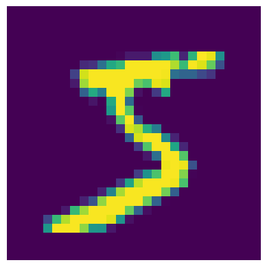
Mnist datasetYou can import Mnist dataset from keras as follow.
from keras.datasets import mnist
(X_train, label_train), (X_test, label_test) = mnist.load_data()
# Visualize
import matplotlib.pyplot as plt
plt.imshow(X_train[0,:,:])
plt.axis("off")
plt.show()
A. What’s the dimension of X_train and X_test?
Can you guess what are label_train and label_test?
How many distinct values of these labels?
# To doB. Visualize the first 8 images of the training data in two rows.
import matplotlib.pyplot as plt
# To do
C. Reshape the training data and testing data from 3 dimensional into 2 dimensional using x.reshape(), i.e., \(n\times 28\times 28\to n\times 784\) where each row is a \(784\)-dimensional vector of each image.
# To doD. Scale the training and testing inputs pixels to take values between \(0\) and \(1\). This helps the training process converges quickly.
# To doHere, we build MLP model with the following architecture and hyperparameters:
A. Designing a network
Let me set up all these for you.
from keras.models import Sequential
from keras.layers import Input, Dense


d = 784 # Input dimensions
M = 10 # Number of classes

model = Sequential()
# input layer
model.add(Input(shape=(d,)))

# Hidden layers
# Add hidden layer of size 32
model.add(Dense(32, activation='relu'))

# Add another hidden layer of size 32
model.add(Dense(32, activation='relu'))

# Add one last layer (output) of size
model.add(Dense(10, activation='softmax'))
# Compiling the model: set up the optimization, loss and metric
from keras.optimizers import Adam, SGD
lr = 0.001
model.compile(
optimizer=SGD(learning_rate=lr),
loss='sparse_categorical_crossentropy',
metrics=['accuracy'])
# Fit the model
b = 32
n_epoch = 50
val_size = 0.2
history = model.fit(X_train, label_train, epochs=n_epoch, batch_size=b, validation_split=val_size)B. Learning curves can be extracted from the history object.
Create learning curves as shown in slide 29.
What information do you get from the curves?
Compute the testing accuracy.
Visualize images that are wrongly predicted.
# To doC. The network’s architecture and hyperparameters were defined nearly at random. Now, it is your turn to try to study the impact of these values.
Increase the number of neurons within each hidden layers.
Change activation function.
Change the learning rate.
Change the optimization algorithm.
Change the minibatch size \(b\).
In each case, compute the test performance of the model.
# To doMnist dataset