TP3 - Deep Neural Networks (DNN)

---

Course: Advanced Machine Learning
Lecturer: Sothea HAS, PhD

Objective: We had studied how to detect the connection between inputs and the target. It is important to truely estimate this connection through various models. This practical session (TP) is designed to familiarize you with concept and application of Deep Neural Networks, which is a powerful model that is theoretically able to reconstruct any reasonably complex input-output relationship.

• The notebook of this TP can be downloaded here: TP3_DNN.ipynb.

---

1. Universal Approximation Theorem

DNNs have been proven to be universal approximators which means that they can approximate any reasonably complex continuous functions.

A. Create your own function \(f\), for example:

\[f(x)=|x|(1+\sin^2(x))+1+\epsilon, \epsilon\sim{\cal N}(0,\sigma^2).\]

• Define python function to evaluate your function \(f\).
• Plot the graph of this function at \(n=1000\) values some domain \(D\), for example \(D=[-5,5]\).

import plotly.io as pio
pio.renderers.default = 'notebook'
# For example
import numpy as np
def f(x):
    return np.abs(x)*(1+np.sin(x) ** 2) + 1

import plotly.graph_objs as go
n = 1000
X = np.linspace(-5,5,n)
val = f(X)
y = val + np.random.normal(0,1, size=n)
fig = go.Figure(go.Scatter(x = X, y = y, mode="markers", name="Data points"))
fig.add_trace(go.Scatter(x=X, y=val, name="True function"))
fig.update_layout(
      title="Data and its underlying function", 
      width=600, height=500,
      xaxis_title=dict(text='x'),
      yaxis_title=dict(text='y=f(x)'))

fig.show()

B. Build a \(2\)-layer DNN with your favorite hyperparameters to estimate this function on the domain \(D\) (You can use your favorite Python modules such as Keras or Pytorch to build the model).

• Vary the hyperparameters such as mini-batch, number of epochs, penalty strength,… of the network for better approximation.

• Plot the learning curves as you make change to the network.

• Plot the fitted curve and compare to the true data above.

• Using the trained network to predict \(x\) outside the domain \(D\), for example, on the interval x_test = np.linspace(5,7,50). What do you observe?

# This is an example with Keras
from sklearn.metrics import mean_squared_error 
from keras.models import Sequential 
from keras.layers import Dense, Input

# Input
d = 1

model = Sequential()
model.add(Input(shape=(d,)))

# To do

C. Increase the number of layers and observe the change in the network approximation power.

• Compare the approximation to the true function.

• Make outside domain prediction. Comment.

2. Heart disease dataset

• Your mission here is to recreate what we had done in the course on the Heart Disease Dataset.

• Report test performance metrics.

import numpy as np
import pandas as pd
import kagglehub
# Download latest version
path = kagglehub.dataset_download("johnsmith88/heart-disease-dataset")
data = pd.read_csv(path + "/heart.csv")
data.head(5)

	age	sex	cp	trestbps	chol	fbs	restecg	thalach	exang	oldpeak	slope	ca	thal	target
0	52	1	0	125	212	0	1	168	0	1.0	2	2	3	0
1	53	1	0	140	203	1	0	155	1	3.1	0	0	3	0
2	70	1	0	145	174	0	1	125	1	2.6	0	0	3	0
3	61	1	0	148	203	0	1	161	0	0.0	2	1	3	0
4	62	0	0	138	294	1	1	106	0	1.9	1	3	2	0

3. Mnist dataset

In this section, you will work with Mnist dataset. It can be imported using the following codes.

from keras.datasets import mnist

(train_images, train_labels), (test_images, test_labels) = mnist.load_data()

import matplotlib.pyplot as plt
import numpy as np
digit = np.random.choice(train_images.shape[0], size=10)
_ , axs = plt.subplots(2,5, figsize=(9, 3))
for i in range(10):
  axs[i//5, i%5].imshow(train_images[digit[i]])
  axs[i//5, i%5].axis("off")
  axs[i//5, i%5].set_title(f"True label: {train_labels[digit[i]]}")
plt.tight_layout()
plt.show()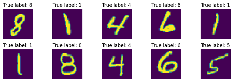

• Build your own designed DNN to identify the digits of testing images.
• Evaluate its performance using suitable matrix and conclude.

# To do

References

\(^{\text{📚}}\) Deep Learning, Ian Goodfellow. (2016)..
\(^{\text{📚}}\) Hands-on ML with Sklearn, Keras & Tensorflow, Aurélien Geron (2017)..
\(^{\text{📚}}\) Heart Disease Dataset.
\(^{\text{📚}}\) Backpropagation, 3B1B.