TP4 - Nonparametric Models

Course: Advanced Machine Learning
Lecturer: Sothea HAS, PhD

Objective: We have seen in the course that nonparametric models aim at directly estimating the regression function of MSE criterion. In this TP, we shall learn how to implement the three basic nonparametric models including \(K\)-NN, Decision Trees and Kernel Smoother method.

The notebook of this TP can be downloaded here: TP4_Nonparametric.ipynb.

1. Abalone Dataset

Abalone is a popular seafood in Japanese and European cuisine. However, the age of abalone is determined by cutting the shell through the cone, staining it, and counting the number of Rings through a microscope, a boring and time-consuming task. Other measurements, which are easier to obtain, are used to predict the age, including their physical measurements, weights etc. This section aims at predicting the Rings of abalone using its physical measurements. Read and load the data from kaggle: Abalone dataset.

# %pip install kagglehub   # if you have not installed "kagglehub" module yet
import kagglehub

# Download latest version
path = kagglehub.dataset_download("rodolfomendes/abalone-dataset")

# Import data
import pandas as pd
data = pd.read_csv(path + "/abalone.csv")
data.head()

	Sex	Length	Diameter	Height	Whole weight	Shucked weight	Viscera weight	Shell weight	Rings
0	M	0.455	0.365	0.095	0.5140	0.2245	0.1010	0.150	15
1	M	0.350	0.265	0.090	0.2255	0.0995	0.0485	0.070	7
2	F	0.530	0.420	0.135	0.6770	0.2565	0.1415	0.210	9
3	M	0.440	0.365	0.125	0.5160	0.2155	0.1140	0.155	10
4	I	0.330	0.255	0.080	0.2050	0.0895	0.0395	0.055	7

A. Overview of the dataset.

What’s the dimension of this dataset? How many quantitative and qualitative variables are there in this dataset?

print(f'Dimension: {data.shape}')
data.dtypes

Dimension: (4177, 9)

Sex                object
Length            float64
Diameter          float64
Height            float64
Whole weight      float64
Shucked weight    float64
Viscera weight    float64
Shell weight      float64
Rings               int64
dtype: object

print(f'Quantitative columns: {data.select_dtypes(include="number").columns}')
print(f'Quantitative columns: {data.select_dtypes(exclude="number").columns}')

Quantitative columns: Index(['Length', 'Diameter', 'Height', 'Whole weight', 'Shucked weight',
       'Viscera weight', 'Shell weight', 'Rings'],
      dtype='object')
Quantitative columns: Index(['Sex'], dtype='object')

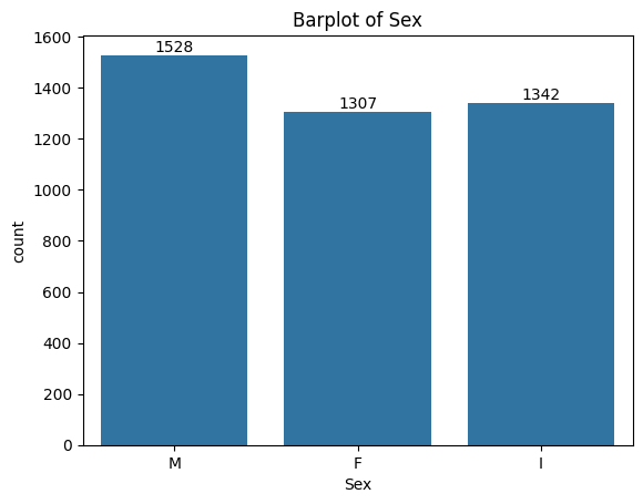
Create statistical summary of the dataset. Identify problems if there is any in this dataset.

# Qualitative data
data[['Sex']].value_counts(normalize=True).to_frame().T

import matplotlib.pyplot as plt
import seaborn as sns
ax = sns.countplot(data, x="Sex")
ax.set_title("Barplot of Sex")
ax.bar_label(ax.containers[0])
plt.show()

data.describe().drop(labels=['count'])

	Length	Diameter	Height	Whole weight	Shucked weight	Viscera weight	Shell weight	Rings
mean	0.523992	0.407881	0.139516	0.828742	0.359367	0.180594	0.238831	9.933684
std	0.120093	0.099240	0.041827	0.490389	0.221963	0.109614	0.139203	3.224169
min	0.075000	0.055000	0.000000	0.002000	0.001000	0.000500	0.001500	1.000000
25%	0.450000	0.350000	0.115000	0.441500	0.186000	0.093500	0.130000	8.000000
50%	0.545000	0.425000	0.140000	0.799500	0.336000	0.171000	0.234000	9.000000
75%	0.615000	0.480000	0.165000	1.153000	0.502000	0.253000	0.329000	11.000000
max	0.815000	0.650000	1.130000	2.825500	1.488000	0.760000	1.005000	29.000000

print(f'Abalone with 0 height: {sum(data.Height == 0)}')
print(f'Number of duplicated data: {sum(data.duplicated())}')

Abalone with 0 height: 2
Number of duplicated data: 0

There are two abalone with 0 heights. We should remove them.

data.query('Height > 0', inplace=True)

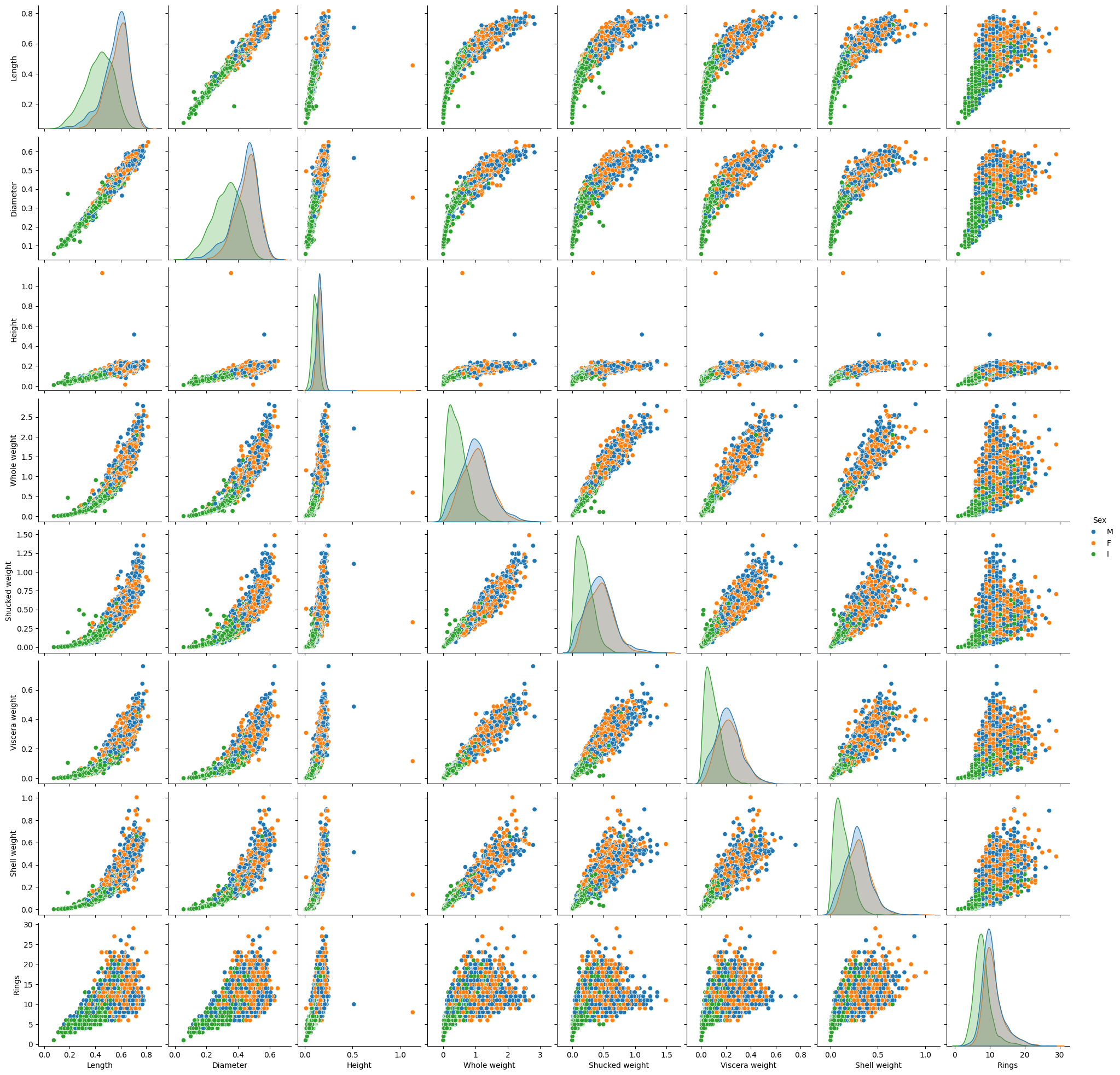
Study the correlation matrix of this dataset. Comment this correlation matrix.

data.select_dtypes(include='number').corr().style.background_gradient()

	Length	Diameter	Height	Whole weight	Shucked weight	Viscera weight	Shell weight	Rings
Length	1.000000	0.986802	0.828108	0.925217	0.897859	0.902960	0.898419	0.556464
Diameter	0.986802	1.000000	0.834298	0.925414	0.893108	0.899672	0.906084	0.574418
Height	0.828108	0.834298	1.000000	0.819886	0.775621	0.798908	0.819596	0.557625
Whole weight	0.925217	0.925414	0.819886	1.000000	0.969389	0.966354	0.955924	0.540151
Shucked weight	0.897859	0.893108	0.775621	0.969389	1.000000	0.931924	0.883129	0.420597
Viscera weight	0.902960	0.899672	0.798908	0.966354	0.931924	1.000000	0.908186	0.503562
Shell weight	0.898419	0.906084	0.819596	0.955924	0.883129	0.908186	1.000000	0.627928
Rings	0.556464	0.574418	0.557625	0.540151	0.420597	0.503562	0.627928	1.000000

Shell weight appears to be the most correlated input with the target. Moreover, there are many highly correlated pairs which might impact performance of the model. Moreover, as the number of inputs is small enough, we can visualize scatter plot of each pairs as follows.

sns.pairplot(data, hue="Sex")
plt.show()

There seems to be outliers in variable height that might impact model performance. Such outliers should be removed.

data.query("Height < 0.5", inplace=True)

B. Model development.

Split the dataset into \(80\%-20\%\) training-testing data using random_state = 42.

from sklearn.model_selection import train_test_split

X_train, X_test, y_train, y_test = train_test_split(
                    data.drop(columns=['Rings']), 
                    data.Rings,
                    test_size=0.2,
                    random_state=42)
print(f'Train size: {X_train.shape}')
print(f'Test size: {X_test.shape}')

Train size: (3338, 8)
Test size: (835, 8)

Build a \(K\)-NN model and fine-tune it to predict the testing data. Report its RMSE.

from sklearn.neighbors import KNeighborsRegressor
from sklearn.model_selection import GridSearchCV
from sklearn.preprocessing import StandardScaler
import numpy as np

# Encode Sex
X_train = pd.concat([
    pd.get_dummies(X_train['Sex'], drop_first=True),
    X_train.drop(columns=['Sex'])], axis=1)
X_test = pd.concat([
    pd.get_dummies(X_test['Sex'], drop_first=True),
    X_test.drop(columns=['Sex'])], axis=1)

scaler = StandardScaler()
X_train_scaled = scaler.fit_transform(X_train)
X_test_scaled = scaler.transform(X_test)
knn = KNeighborsRegressor()
param = {
    "n_neighbors": np.arange(1, 15, 1)
}

grid_cv = GridSearchCV(knn, param, cv=10, scoring="neg_mean_squared_error", verbose=1)
grid_cv = grid_cv.fit(X_train_scaled, y_train)

Fitting 10 folds for each of 14 candidates, totalling 140 fits

print(f'Best number of neighbors: {grid_cv.best_params_}')
knn = grid_cv.best_estimator_.fit(X_train_scaled, y_train)
y_pred = knn.predict(X_test_scaled)

from sklearn.metrics import mean_absolute_error, r2_score

print(f'Test RMSE: {np.sqrt(mean_absolute_error(y_test, y_pred))}')

import plotly.graph_objects as go
fig = go.Figure(go.Scatter(x=y_test, y=y_pred, name="Actual vs Pred", mode="markers", marker=dict(size=10)))
fig.add_trace(go.Scatter(x=y_test, y=y_test, name="Line y = x", mode="lines", line=dict(color='red')))
fig.update_layout(height=500, width=700, title="Actual vs Prediction")
fig.show()

Best number of neighbors: {'n_neighbors': 12}
Test RMSE: 1.2482722590583077

Unable to display output for mime type(s): application/vnd.plotly.v1+json

Build a Regression Tree to predict the testing data and report its RMSE.

from sklearn.tree import DecisionTreeRegressor
param = {
    'min_samples_leaf' : [15,20,30, 40, 50],
    'criterion': ['squared_error', 'absolute_error'],
    'min_samples_split': [5, 8, 10, 15, 20],
    'max_features': [5,6,7,8]
}

tr = DecisionTreeRegressor()
grid_cv = GridSearchCV(tr, param, cv=10)
grid_cv = grid_cv.fit(X_train, y_train)

print(f'Best tree hyperparameters: {grid_cv.best_params_}')
tr = grid_cv.best_estimator_.fit(X_train, y_train)
y_pred_tr = tr.predict(X_test)

print(f'Test RMSE: {np.sqrt(mean_absolute_error(y_test, y_pred_tr))}')

import plotly.graph_objects as go
fig1 = go.Figure(go.Scatter(x=y_test, y=y_pred_tr, name="Actual vs Pred", mode="markers", marker=dict(size=10)))
fig1.add_trace(go.Scatter(x=y_test, y=y_test, name="Line y = x", mode="lines", line=dict(color='red')))
fig1.update_layout(height=500, width=700, title="Actual vs Prediction")
fig1.show()

Best tree hyperparameters: {'criterion': 'squared_error', 'max_features': 8, 'min_samples_leaf': 20, 'min_samples_split': 20}
Test RMSE: 1.294609989247988

Unable to display output for mime type(s): application/vnd.plotly.v1+json

Build a Kernel Smoother method to predict the testing data and report its RMSE (my python module: gradientcobra and its module: KernelSmoother).

from gradientcobra.gradientcobra import KernelSmoother

ks = KernelSmoother(
    bandwidth_list=np.linspace(
        1, 10, num=300), 
    opt_method="grid",
    norm_constant=30)
ks = ks.fit(X_train_scaled, y_train)

* Grid search progress: 100%|██████████| 300/300 [02:23<00:00,  2.10it/s]

print(f'Best smoothing parameter: {ks.optimization_outputs['opt_bandwidth']}')
ks.draw_learning_curve()

Best smoothing parameter: [7.62207358]

Let’s see how the quality of the model.

y_pred_ks = ks.predict(X_test_scaled)

print(f'Test RMSE: {np.sqrt(mean_absolute_error(y_test, y_pred_ks))}')

import plotly.graph_objects as go
fig2 = go.Figure(go.Scatter(x=y_test, y=y_pred_ks, name="Actual vs Pred", mode="markers", marker=dict(size=10)))
fig2.add_trace(go.Scatter(x=y_test, y=y_test, name="Line y = x", mode="lines", line=dict(color='red')))
fig2.update_layout(height=500, width=700, title="Actual vs Prediction")
fig2.show()

Test RMSE: 1.2501940214421492

C. Neural Network.

Design a neural network to predict the testing data and compute its RMSE.
Compre to the previous results and conclude.

# This is an example with Keras
from sklearn.metrics import mean_squared_error
from keras.models import Sequential
from keras.layers import Dense, Input
from keras import regularizers

# Input
d = X_train.shape[1]

model = Sequential()
model.add(Input(shape=(d,)))

model.add(Dense(64, activation="relu"))
model.add(Dense(64, activation="relu"))
model.add(Dense(1, activation="linear"))

# Set up optimizer for our model
model.compile(optimizer='adam', loss='mean_squared_error', metrics=['mse'])

# Training the network
history = model.fit(
    X_train_scaled, 
    y_train, 
    epochs=100, 
    batch_size=32, 
    validation_split=0.1, 
    verbose=0)

# Extract loss values
train_loss = history.history['loss']
val_loss = history.history['val_loss']

import plotly.io as pio
pio.renderers.default = 'notebook'

# Plot the learning curves
epochs = list(range(1, len(train_loss) + 1))
fig1 = go.Figure(go.Scatter(x=epochs, y=train_loss, name="Training loss"))
fig1.add_trace(go.Scatter(x=epochs, y=val_loss, name="Training loss"))
fig1.update_layout(title="Training and Validation Loss",
                   width=800, height=500,
                   xaxis=dict(title="Epoch", type="log"),
                   yaxis=dict(title="Loss"))
fig1.show()

y_pred_nn = model.predict(X_test_scaled)

print(f'Test RMSE: {np.sqrt(mean_absolute_error(y_test, y_pred_nn))}')

import plotly.graph_objects as go
fig2 = go.Figure(go.Scatter(x=y_test, y=y_pred_nn.reshape(-1), name="Actual vs Pred", mode="markers", marker=dict(size=10)))
fig2.add_trace(go.Scatter(x=y_test, y=y_test, name="Line y = x", mode="lines", line=dict(color='red')))
fig2.update_layout(height=500, width=700, title="Actual vs Prediction")
fig2.show()

27/27 ━━━━━━━━━━━━━━━━━━━━ 0s 6ms/step
Test RMSE: 1.2237433819694146

2. Revisit `Spam` dataset

Your task in this section is to create email spam filters by applying the nonparametric models introduced in the course.
Report test performance metrics on the spam dataset loaded below.
Build a pipeline that takes text input as a real email, then return the type of the email using your best spam filter found in the first question.

path = "https://raw.githubusercontent.com/hassothea/MLcourses/main/data/spam.txt"
data = pd.read_csv(path, sep=" ")

from sklearn.preprocessing import MinMaxScaler

X_train, X_test, y_train, y_test = train_test_split(
    data.iloc[:,1:-1],
    data['type'],
    test_size=0.2,
    random_state=42)

scaler = MinMaxScaler()
X_train_scaled = scaler.fit_transform(X_train)
X_test_scaled = scaler.transform(X_test)

# One-hot encoding
encode = {"spam": 1, "nonspam": 0}
decode = {0: "nonspam", 1: "spam"}
# y_train = np.array([encode[i] for i in y_train])
# y_test = np.array([encode[i] for i in y_test])

data.head(5)

	Id	make	address	all	our	over	remove	internet	order	...	charSemicolon	charRoundbracket	charExclamation	charDollar	charHash	capitalAve	capitalLong	capitalTotal	type
0	1	0.00	0.64	0.64	0.32	0.00	0.00	0.00	0.00	...	0.00	0.000	0.778	0.000	0.000	3.756	61	278	spam
1	2	0.21	0.28	0.50	0.14	0.28	0.21	0.07	0.00	...	0.00	0.132	0.372	0.180	0.048	5.114	101	1028	spam
2	3	0.06	0.00	0.71	1.23	0.19	0.19	0.12	0.64	...	0.01	0.143	0.276	0.184	0.010	9.821	485	2259	spam
3	4	0.00	0.00	0.00	0.63	0.00	0.31	0.63	0.31	...	0.00	0.137	0.137	0.000	0.000	3.537	40	191	spam
4	5	0.00	0.00	0.00	0.63	0.00	0.31	0.63	0.31	...	0.00	0.135	0.135	0.000	0.000	3.537	40	191	spam

5 rows × 59 columns

We perform Cross-validation on KNN

from sklearn.neighbors import KNeighborsClassifier
from sklearn.metrics import confusion_matrix
knn = KNeighborsClassifier()
param = {
    "n_neighbors": np.arange(1, 40, 1)
}

grid_cv = GridSearchCV(knn, param, cv=10, scoring="neg_log_loss", verbose=0)
grid_cv = grid_cv.fit(X_train_scaled, y_train)

print(f'Best number of neighbors: {grid_cv.best_params_}')
knn = grid_cv.best_estimator_.fit(X_train_scaled, y_train)
y_pred = knn.predict(X_test_scaled)

print(f'Accuracy: {np.mean(y_test == y_pred)}')
confusion_matrix(y_test, y_pred)

Best number of neighbors: {'n_neighbors': 29}
Accuracy: 0.8718783930510315

array([[500,  31],
       [ 87, 303]], dtype=int64)

from sklearn.tree import DecisionTreeClassifier


tr = DecisionTreeClassifier()
param = {
    'min_samples_leaf' : [45,50,55,60,65, 70, 75, 80],
    'criterion': ['entropy', 'gini'],
    'min_samples_split': [5, 8, 10, 12, 15, 18, 20],
    'max_features': np.arange(1,50, 10)
}

grid_cv = GridSearchCV(tr, param, cv=10, scoring="neg_log_loss", verbose=0)
grid_cv = grid_cv.fit(X_train, y_train)

print(f'Best number of neighbors: {grid_cv.best_params_}')
tr = grid_cv.best_estimator_.fit(X_train, y_train)
y_pred = tr.predict(X_test)

print(f'Accuracy: {np.mean(y_test == y_pred)}')
confusion_matrix(y_test, y_pred)

Best number of neighbors: {'criterion': 'entropy', 'max_features': 31, 'min_samples_leaf': 65, 'min_samples_split': 10}
Accuracy: 0.8957654723127035

array([[500,  31],
       [ 65, 325]], dtype=int64)

We can build a Pipeline that converts real emails to be a data frame of consistent format for our models.

def SpamFilter(email, method = "knn"):
    def capitals(text, count, symbol):
        total_capitals = 0
        longest_sequence = 0
        current_sequence = 0
        capital_lengths = []
        sym = set(symbol)
        for char in text:
            if char.lower() in sym:
                count[symbol[char]] += 1
            elif char in count.keys():
                count[char] += 1
            if char.isupper():
                total_capitals += 1
                current_sequence += 1
            else:
                if current_sequence > 0:
                    capital_lengths.append(current_sequence)
                    if current_sequence > longest_sequence:
                        longest_sequence = current_sequence
                    current_sequence = 0

        # Append the last sequence if it ends with a capital letter
        if current_sequence > 0:
            capital_lengths.append(current_sequence)
            if current_sequence > longest_sequence:
                longest_sequence = current_sequence

        average_length = sum(capital_lengths) / len(capital_lengths) if capital_lengths else 0
        count['capitalTotal'], count['capitalLong'], count['capitalAve'] = total_capitals, longest_sequence, average_length

        return count

    symbol = {
        '000': 'num000',
        '650': 'num650',
        '857': 'num857',
        '415': 'num415',
        '85': 'num85',
        '1999': 'num1999',
        ';': 'charSemicolon',
        '(': 'charRoundbracket',
        ')': 'charRoundbracket',
        '[': 'charSquarebracket',
        ']': 'charSquarebracket',
        '!': 'charExclamation',
        '$': 'charDollar',
        '#': 'charHash'}
    count = {x: 0 for x in data.columns[1:-1]}
    count_ = capitals(email, count, symbol)
    X = pd.DataFrame(count_, index=[0])
    X = scaler.transform(X)
    if method == "knn":
        pred = knn.predict(X)
    else:
        pred = tr.predict(X)
    return pred[0]

# test
email = 'Hi Jack,\n I hope this email find you well. I am writing to ask for the address of Marry because I want to send her an invitation for my wedding.\n\n Thank you for the information.\n\n Best regards, Mark'

# This is the prediction by KNN
print(f'KNN predict this email to be: {SpamFilter(email)}')

# This is the prediction by Tree
print(f'Tree predict this email to be: {SpamFilter(email)}')

KNN predict this email to be: nonspam
Tree predict this email to be: nonspam

References

\(^{\text{📚}}\) The Element of Statistical Learning, Hastie et al. (2002).
\(^{\text{📚}}\) A Distribution-free Theory of Nonparameteric Regression, Györfi et al. (2002)..
\(^{\text{📚}}\) A Probabilistic Theory of Pattern Recognition, Devroye et al. (1997).

1. Abalone Dataset

2. Revisit Spam dataset

References

2. Revisit `Spam` dataset