TP3 - Deep Neural Networks (DNN)

Course: Advanced Machine Learning
Lecturer: Sothea HAS, PhD

Objective: We had studied how to detect the connection between inputs and the target. It is important to truely estimate this connection through various models. This practical session (TP) is designed to familiarize you with concept and application of Deep Neural Networks, which is a powerful model that is theoretically able to reconstruct any reasonably complex input-output relationship.

The notebook of this TP can be downloaded here: TP3_DNN.ipynb.

1. Universal Approximation Theorem

DNNs have been proven to be universal approximators which means that they can approximate any reasonably complex continuous functions.

A. Create your own function \(f\), for example:

\[f(x)=|x|(1+\sin^2(x))+1+\epsilon, \epsilon\sim{\cal N}(0,\sigma^2).\]

Define python function to evaluate your function \(f\).
Plot the graph of this function at \(n=1000\) values some domain \(D\), for example \(D=[-5,5]\).

import plotly.io as pio
pio.renderers.default = 'notebook'
# For example
import numpy as np
def f(x):
    return np.abs(x)*(1+np.sin(x) ** 2) + 1

import plotly.graph_objs as go
n = 1000
X = np.linspace(-5,5,n)
val = f(X)
y = val + np.random.normal(0,1, size=n)
fig = go.Figure(go.Scatter(x = X, y = y, mode="markers", name="Data points"))
fig.add_trace(go.Scatter(x=X, y=val, name="True function"))
fig.update_layout(
      title="Data and its underlying function",
      width=800, height=500,
      xaxis_title=dict(text='x'),
      yaxis_title=dict(text='y=f(x)'))

fig.show()

B. Build a \(2\)-layer DNN with your favorite hyperparameters to estimate this function on the domain \(D\) (You can use your favorite Python modules such as Keras or Pytorch to build the model).

Vary the hyperparameters such as mini-batch, number of epochs, penalty strength,… of the network for better approximation.
Plot the learning curves as you make change to the network.
Plot the fitted curve and compare to the true data above.

# This is an example with Keras
from sklearn.metrics import mean_squared_error
from keras.models import Sequential
from keras.layers import Dense, Input
from keras import regularizers

# Input
d = 1

model = Sequential()
model.add(Input(shape=(d,)))

# To do
model.add(Dense(64, activation="relu"))
model.add(Dense(64, activation="relu"))
model.add(Dense(1, activation="linear"))

# Set up optimizer for our model
model.compile(optimizer='adam', loss='mean_squared_error', metrics=['mse'])

# Training the network
history = model.fit(X, y, epochs=2000, batch_size=32, validation_split=0.1, verbose=0)

# Extract loss values
train_loss = history.history['loss']
val_loss = history.history['val_loss']

import plotly.io as pio
pio.renderers.default = 'notebook'

# Plot the learning curves
epochs = list(range(1, len(train_loss) + 1))
fig1 = go.Figure(go.Scatter(x=epochs, y=train_loss, name="Training loss"))
fig1.add_trace(go.Scatter(x=epochs, y=val_loss, name="Training loss"))
fig1.update_layout(title="Training and Validation Loss",
                   width=800, height=500,
                   xaxis=dict(title="Epoch", type="log"),
                   yaxis=dict(title="Loss"))
fig1.show()

import plotly.io as pio
pio.renderers.default = 'notebook'

from sklearn.metrics import mean_squared_error

y_pred = model.predict(X)
print(f'MSE: {mean_squared_error(y, y_pred)/np.mean(y) ** 2}')

fig_pred = go.Figure(data=[
    fig.data[0],
    fig.data[1]
])
fig_pred.add_trace(go.Scatter(x=X, y=y_pred.reshape(-1), mode='lines', name="prediction", line=dict(color="green")))
fig_pred.update_layout(width = 800, height= 600, title="True vs Prediction")
fig_pred.show()

32/32 ━━━━━━━━━━━━━━━━━━━━ 0s 4ms/step
MSE: 0.039028134998251314

Using the trained network to predict \(x\) outside the domain \(D\), for example, on the interval x_test = np.linspace(5,7,50). What do you observe?

import plotly.io as pio
pio.renderers.default = 'notebook'

x_full = np.linspace(-5, 8, 100)
x_new = np.linspace(-5, 5, 100)
x_out = np.linspace(5,  8, 100)
y_new = model.predict(x_new).reshape(-1)
y_out = model.predict(x_out).reshape(-1)
fig_out = go.Figure(go.Scatter(x=x_full, y=f(x_full), name="True function"))
fig_out.add_trace(go.Scatter(x=x_new, y=y_new, name="On-domain predictions", line=dict(color="red")))
fig_out.add_trace(go.Scatter(x=x_out, y=y_out, name="Outside domain predictions", line=dict(color="green", dash = "dash")))
fig_out.update_layout(width=800, height=600, title='Outside domain prediction', xaxis = dict(title="x"), yaxis=dict(title="y"))
fig_out.show()

4/4 ━━━━━━━━━━━━━━━━━━━━ 0s 14ms/step
4/4 ━━━━━━━━━━━━━━━━━━━━ 0s 13ms/step

Neural networks are decompositions of matrix multiplications and some nonlinear activation functions. It learns by adjusting weights and biases to minimize loss function. The resulting network is not the true input-output relationship on the entire domain but the approximation of what it has seen within the given range of inputs. The generalization to outside domain/range is poor because, by construction, its true nature is almost linear from some threshold of inputs (outside domain). In other words, it’s poor at extrapolating but great at interpolating.

Let’s try to modify some hyperparameters and observe the performance of the network.
- Noramlly, increase batch size has similar effect as decaying learning rate (see: Smith et al. (2018)). We shall explore that with the number of epoches.

# We setup a model with 3 hidden layers
model = Sequential()
model.add(Input(shape=(d,)))

# To do
model.add(Dense(64, activation="relu"))
model.add(Dense(64, activation="relu"))
model.add(Dense(1, activation="linear"))

# Set up optimizer for our model
model.compile(optimizer='adam', loss='mean_squared_error', metrics=['mse'])

# Training the network
history = model.fit(X, y, epochs=2000, batch_size=120, validation_split=0.1, verbose=0)

# Extract loss values
train_loss = history.history['loss']
val_loss = history.history['val_loss']

import plotly.io as pio
pio.renderers.default = 'notebook'

# Plot the learning curves
epochs = list(range(1, len(train_loss) + 1))
fig1 = go.Figure(go.Scatter(x=epochs, y=train_loss, name="Training loss"))
fig1.add_trace(go.Scatter(x=epochs, y=val_loss, name="Training loss"))
fig1.update_layout(title="Training and Validation Loss",
                   width=800, height=500,
                   xaxis=dict(title="Epoch", type="log"),
                   yaxis=dict(title="Loss"))

import plotly.io as pio
pio.renderers.default = 'notebook'

x_full = np.linspace(-5, 8, 100)
x_new = np.linspace(-5, 5, 100)
x_out = np.linspace(5,  8, 100)
y_new = model.predict(x_new).reshape(-1)
y_out = model.predict(x_out).reshape(-1)
fig_out = go.Figure(go.Scatter(x=x_full, y=f(x_full), name="True function"))
fig_out.add_trace(go.Scatter(x=x_new, y=y_new, name="On-domain predictions", line=dict(color="red")))
fig_out.add_trace(go.Scatter(x=x_out, y=y_out, name="Outside domain predictions", line=dict(color="green", dash = "dash")))
fig_out.update_layout(width=800, height=600, title='Outside domain prediction', xaxis = dict(title="x"), yaxis=dict(title="y"))
fig_out.show()

4/4 ━━━━━━━━━━━━━━━━━━━━ 0s 44ms/step
4/4 ━━━━━━━━━━━━━━━━━━━━ 0s 14ms/step

The learning curve suggests that the validation curve converges more slowly torwards the stable region compared to the previous case. This is what we would observe with small learning rate. However, increasing batch size provides more stable learning process than the case of small batch size and small learning rate.

Let’s increase the number of neurons.

# We setup a model with 3 hidden layers
model = Sequential()
model.add(Input(shape=(d,)))

# To do
model.add(Dense(128, activation="relu"))
model.add(Dense(128, activation="relu"))
model.add(Dense(1, activation="linear"))

# Set up optimizer for our model
model.compile(optimizer='adam', loss='mean_squared_error', metrics=['mse'])

# Training the network
history = model.fit(X, y, epochs=2000, batch_size=120, validation_split=0.1, verbose=0)

# Extract loss values
train_loss = history.history['loss']
val_loss = history.history['val_loss']

import plotly.io as pio
pio.renderers.default = 'notebook'

# Plot the learning curves
epochs = list(range(1, len(train_loss) + 1))
fig1 = go.Figure(go.Scatter(x=epochs, y=train_loss, name="Training loss"))
fig1.add_trace(go.Scatter(x=epochs, y=val_loss, name="Training loss"))
fig1.update_layout(title="Training and Validation Loss",
                   width=800, height=500,
                   xaxis=dict(title="Epoch", type="log"),
                   yaxis=dict(title="Loss"))

import plotly.io as pio
pio.renderers.default = 'notebook'

x_full = np.linspace(-5, 8, 100)
x_new = np.linspace(-5, 5, 100)
x_out = np.linspace(5,  8, 100)
y_new = model.predict(x_new).reshape(-1)
y_out = model.predict(x_out).reshape(-1)
fig_out = go.Figure(go.Scatter(x=x_full, y=f(x_full), name="True function"))
fig_out.add_trace(go.Scatter(x=x_new, y=y_new, name="On-domain predictions", line=dict(color="red")))
fig_out.add_trace(go.Scatter(x=x_out, y=y_out, name="Outside domain predictions", line=dict(color="green", dash = "dash")))
fig_out.update_layout(width=800, height=600, title='Outside domain prediction', xaxis = dict(title="x"), yaxis=dict(title="y"))
fig_out.show()

4/4 ━━━━━━━━━━━━━━━━━━━━ 0s 28ms/step
4/4 ━━━━━━━━━━━━━━━━━━━━ 0s 13ms/step

C. Increase the number of layers and observe the change in the network approximation power.

Compare the approximation to the true function.
Make outside domain prediction. Comment.

# We setup a model with 3 hidden layers
model = Sequential()
model.add(Input(shape=(d,)))

# To do
model.add(Dense(128, activation="relu"))
model.add(Dense(128, activation="relu"))
model.add(Dense(128, activation="relu"))
model.add(Dense(1, activation="linear"))

# Set up optimizer for our model
model.compile(optimizer='adam', loss='mean_squared_error', metrics=['mse'])

# Training the network
history = model.fit(X, y, epochs=2000, batch_size=128, validation_split=0.1, verbose=0)

# Extract loss values
train_loss = history.history['loss']
val_loss = history.history['val_loss']

The learning curves

import plotly.io as pio
pio.renderers.default = 'notebook'

# Plot the learning curves
epochs = list(range(1, len(train_loss) + 1))
fig2 = go.Figure(go.Scatter(x=epochs, y=train_loss, name="Training loss"))
fig2.add_trace(go.Scatter(x=epochs, y=val_loss, name="Training loss"))
fig2.update_layout(title="Training and Validation Loss",
                   width=800, height=500,
                   xaxis=dict(title="Epoch", type="log"),
                   yaxis=dict(title="Loss"))
fig2.show()

import plotly.io as pio
pio.renderers.default = 'notebook'

y_new2 = model.predict(x_new).reshape(-1)
y_out2 = model.predict(x_out).reshape(-1)
fig_out2 = go.Figure(go.Scatter(x=x_full, y=f(x_full), name="True function"))
fig_out2.add_trace(go.Scatter(x=x_new, y=y_new2, name="On-domain predictions", line=dict(color="red")))
fig_out2.add_trace(go.Scatter(x=x_out, y=y_out2, name="Outside domain predictions", line=dict(color="green", dash = "dash")))
fig_out2.update_layout(width=800, height=600, title='Outside domain prediction', xaxis = dict(title="x"), yaxis=dict(title="y"))
fig_out2.show()

4/4 ━━━━━━━━━━━━━━━━━━━━ 0s 23ms/step 
4/4 ━━━━━━━━━━━━━━━━━━━━ 0s 11ms/step

Let’s train the network even longer, we would like to see if the network overfit the data.

# We setup a model with 3 hidden layers
model = Sequential()
model.add(Input(shape=(d,)))

# To do
model.add(Dense(128, activation="relu"))
model.add(Dense(128, activation="relu"))
model.add(Dense(128, activation="relu"))
model.add(Dense(1, activation="linear"))


# We use Adam optimizer

# Set up optimizer for our model
model.compile(optimizer='adam', loss='mean_squared_error', metrics=['mse'])

# Training the network
history = model.fit(X, y, epochs=5000, batch_size=128, validation_split=0.1, verbose=0)

# Extract loss values
train_loss = history.history['loss']
val_loss = history.history['val_loss']

import plotly.io as pio
pio.renderers.default = 'notebook'

# Plot the learning curves
epochs = list(range(1, len(train_loss) + 1))
fig3 = go.Figure(go.Scatter(x=epochs, y=train_loss, name="Training loss"))
fig3.add_trace(go.Scatter(x=epochs, y=val_loss, name="Training loss"))
fig3.update_layout(title="Training and Validation Loss",
                   width=800, height=500,
                   xaxis=dict(title="Epoch", type="log"),
                   yaxis=dict(title="Loss"))
fig3.show()

import plotly.io as pio
pio.renderers.default = 'notebook'

y_new3 = model.predict(x_new).reshape(-1)
y_out3 = model.predict(x_out).reshape(-1)
fig_out3 = go.Figure(go.Scatter(x=x_full, y=f(x_full), name="True function"))
fig_out3.add_trace(go.Scatter(x=x_new, y=y_new3, name="On-domain predictions", line=dict(color="red")))
fig_out3.add_trace(go.Scatter(x=x_out, y=y_out3, name="Outside domain predictions", line=dict(color="green", dash = "dash")))
fig_out3.update_layout(width=800, height=600, title='Outside domain prediction', xaxis = dict(title="x"), yaxis=dict(title="y"))
fig_out3.show()

4/4 ━━━━━━━━━━━━━━━━━━━━ 0s 25ms/step
4/4 ━━━━━━━━━━━━━━━━━━━━ 0s 8ms/step

We observe that the network barely overfits the data probably due to symmetric noise with constant variance.

2. Heart disease dataset

Your mission here is to recreate what we had done in the course on the Heart Disease Dataset.
Report test performance metrics.

import numpy as np
import pandas as pd
import kagglehub
# Download latest version
path = kagglehub.dataset_download("johnsmith88/heart-disease-dataset")
data = pd.read_csv(path + "/heart.csv")
data.head(5)

	age	sex	trestbps	chol	fbs	restecg	thalach	exang	oldpeak	slope	ca	thal
0	52	1	125	212	0	1	168	0	1.0	2	2	3
1	53	1	140	203	1	0	155	1	3.1	0	0	3
2	70	1	145	174	0	1	125	1	2.6	0	0	3
3	61	1	148	203	0	1	161	0	0.0	2	1	3
4	62	0	138	294	1	1	106	0	1.9	1	3	2

This can be found in the course: Deep Learning.

3. Mnist dataset

In this section, you will work with Mnist dataset. It can be imported using the following codes.

from keras.datasets import mnist
(train_images, train_labels), (test_images, test_labels) = mnist.load_data()

import matplotlib.pyplot as plt
import numpy as np
digit = np.random.choice(train_images.shape[0], size=10)
_ , axs = plt.subplots(2,5, figsize=(9, 3))
for i in range(10):
  axs[i//5, i%5].imshow(train_images[digit[i]])
  axs[i//5, i%5].axis("off")
  axs[i//5, i%5].set_title(f"True label: {train_labels[digit[i]]}")
plt.tight_layout()
plt.show()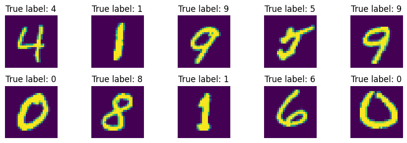

Build your own designed DNN to identify the digits of testing images.
Evaluate its performance using suitable matrix and conclude.

# Processing the data
train_images = train_images.reshape((60000, 28 * 28))
train_images = train_images.astype("float32") / 255
test_images = test_images.reshape((10000, 28 * 28))
test_images = test_images.astype("float32") / 255

print(f'Train images shape: {train_images.shape}')
print(f'Train labels shape: {train_labels.shape}')

from tensorflow.keras.utils import to_categorical

train_labels = to_categorical(train_labels)
test_labels = to_categorical(test_labels)

Train images shape: (60000, 784)
Train labels shape: (60000,)

# We setup a model with 3 hidden layers
model = Sequential()
model.add(Input(shape=(train_images.shape[1],)))

# To do
model.add(Dense(128, activation="relu"))
model.add(Dense(128, activation="relu"))
model.add(Dense(128, activation="relu"))
model.add(Dense(10, activation="softmax"))

# Set up optimizer for our model
model.compile(optimizer='adam', loss='categorical_crossentropy', metrics=['accuracy'])

# Training the network
history = model.fit(train_images, train_labels, epochs=50, batch_size=200, validation_split=0.1, verbose=0)

# Extract loss values
train_loss = history.history['loss']
val_loss = history.history['val_loss']

import plotly.io as pio
pio.renderers.default = 'notebook'

# Plot the learning curves
epochs = list(range(1, len(train_loss) + 1))
fig3 = go.Figure(go.Scatter(x=epochs, y=train_loss, name="Training loss"))
fig3.add_trace(go.Scatter(x=epochs, y=val_loss, name="Training loss"))
fig3.update_layout(title="Training and Validation Loss on Mnist dataset",
                   width=800, height=500,
                   xaxis=dict(title="Epoch", type="log"),
                   yaxis=dict(title="Loss"))

# Test accuracy
pred_test = model.predict(test_images).argmax(axis=1)
true_test = test_labels.argmax(axis=1)
print(f'Test accuracy on Mnist: {np.mean(pred_test==true_test)}')

313/313 ━━━━━━━━━━━━━━━━━━━━ 0s 1ms/step
Test accuracy on Mnist: 0.9839

Let’s see how the mispredicted digits look like.

_ , axs = plt.subplots(2,5, figsize=(15, 5))
mispredicted_id = np.where(pred_test!=true_test)[0]
test_images = test_images.reshape(10000, 28, 28)
for i in range(10):
  axs[i//5, i%5].imshow(test_images[mispredicted_id[i],:,:])
  axs[i//5, i%5].axis("off")
  axs[i//5, i%5].set_title(f"True label: {true_test[mispredicted_id[i]]}; Pred: {pred_test[mispredicted_id[i]]}")
plt.tight_layout()
plt.show()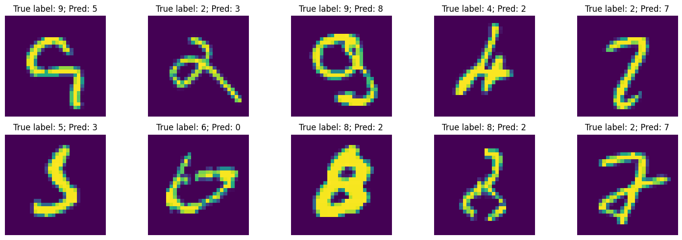

References

\(^{\text{📚}}\) Deep Learning, Ian Goodfellow. (2016)..
\(^{\text{📚}}\) Hands-on ML with Sklearn, Keras & Tensorflow, Aurélien Geron (2017)..
\(^{\text{📚}}\) Heart Disease Dataset.
\(^{\text{📚}}\) Backpropagation, 3B1B.

	age	sex	trestbps	chol	fbs	restecg	thalach	exang	oldpeak	slope	ca	thal
0	52	1	125	212	0	1	168	0	1.0	2	2	3
1	53	1	140	203	1	0	155	1	3.1	0	0	3
2	70	1	145	174	0	1	125	1	2.6	0	0	3
3	61	1	148	203	0	1	161	0	0.0	2	1	3
4	62	0	138	294	1	1	106	0	1.9	1	3	2

	age	sex	trestbps	chol	fbs	restecg	thalach	exang	oldpeak	slope	ca	thal
0	52	1	125	212	0	1	168	0	1.0	2	2	3
1	53	1	140	203	1	0	155	1	3.1	0	0	3
2	70	1	145	174	0	1	125	1	2.6	0	0	3
3	61	1	148	203	0	1	161	0	0.0	2	1	3
4	62	0	138	294	1	1	106	0	1.9	1	3	2

	age	sex	trestbps	chol	fbs	restecg	thalach	exang	oldpeak	slope	ca	thal
0	52	1	125	212	0	1	168	0	1.0	2	2	3
1	53	1	140	203	1	0	155	1	3.1	0	0	3
2	70	1	145	174	0	1	125	1	2.6	0	0	3
3	61	1	148	203	0	1	161	0	0.0	2	1	3
4	62	0	138	294	1	1	106	0	1.9	1	3	2