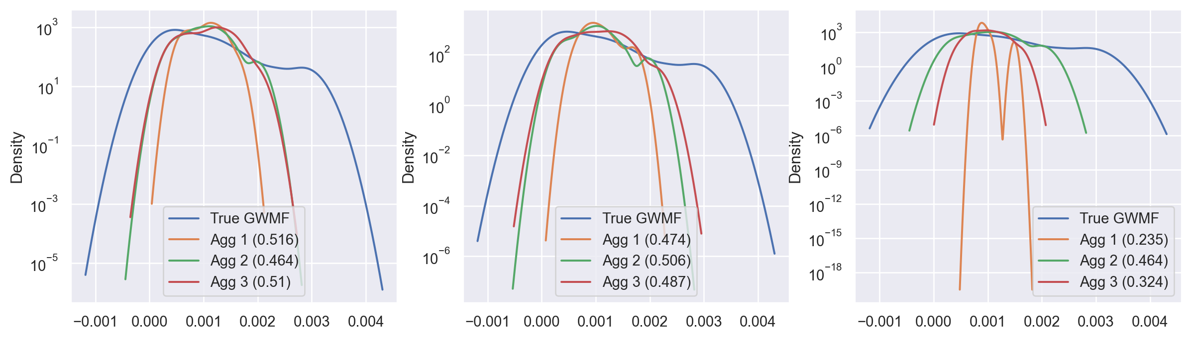
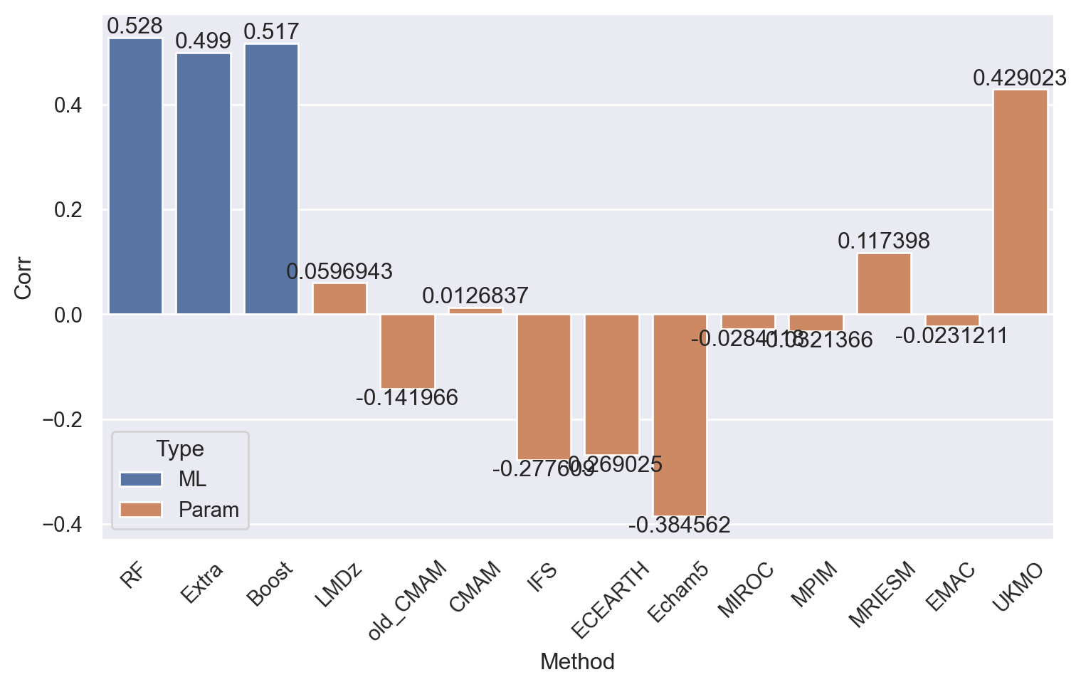
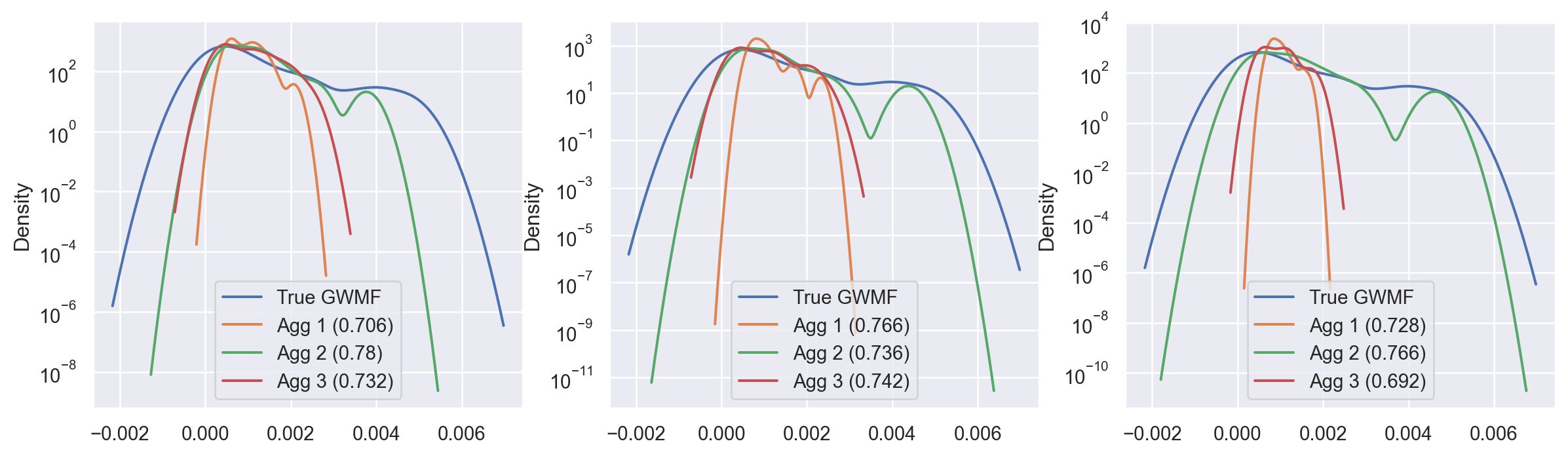
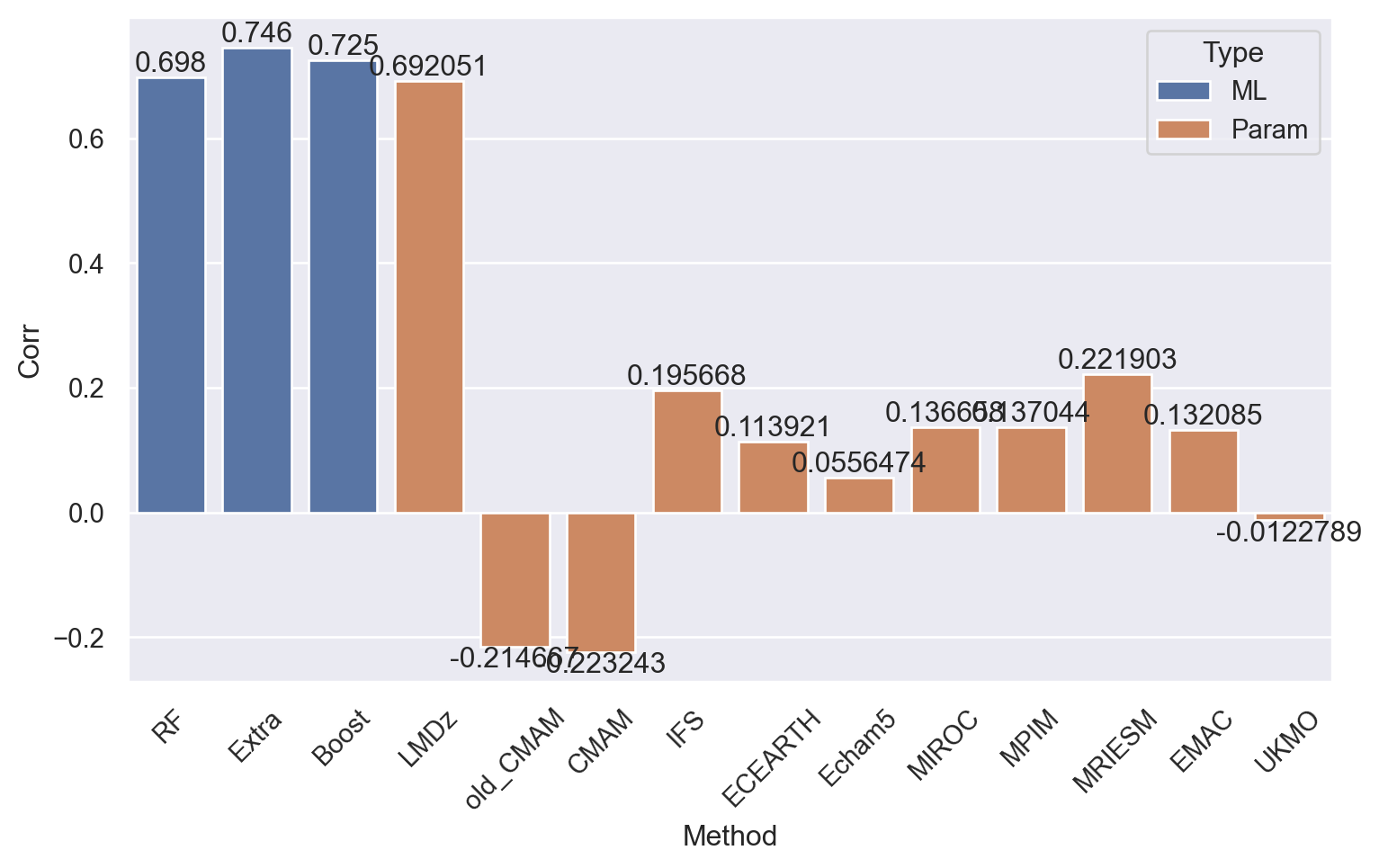
--- title: "Aggregation of ML and Parametrization (2019)" author: "[`Sothea HAS`](https://hassothea.github.io/)" format: html: anchor-sections: true code-tools: true code-fold: true toc: false toc-depth: 3 jupyter: python3 --- # Installing and importing packages ```{python} import sys import netCDF4import xarray as xrimport numpy as npimport matplotlib.pyplot as pltfrom scipy.stats import gaussian_kde as kdeimport pandas as pdimport plotly.graph_objects as gofrom sklearn.preprocessing import StandardScaler, MinMaxScalerimport seaborn as sns``` # Aggregation 1: 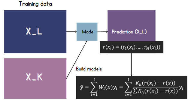 {width="1000px"}# Aggregation 2: 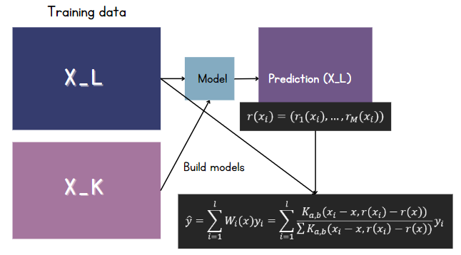 {width="1000px"}# Aggregation 3:  {width="1000px"}# Report result - The first graphic: time series of true gravity wave momentum fluxes and the three aggregation methods.- The second graphic: PDF of the shown time series (logarithmic scale on the y axis).- The barplot of correlations of the 3 ML methods and the 11 parametrizations.```{python} def av_resolution(resulution, y):= len (y) // resulution= len (y) % aif r < resulution/ 2 := np.concatenate((np.repeat(list (range (0 ,a)), resulution), np.repeat(a- 1 , r)))else := np.concatenate((np.repeat(list (range (0 ,a)), resulution), np.repeat(a, r)))return y.groupby(by = group).mean()``` ```{python} #| warning: false #| messages: false from plotly.subplots import make_subplotsimport plotly.graph_objects as go# ml_coef = { # '1' : [0.56, 0.57, 0.58], # '2' : [0.70, 0.67, 0.74], # '3' : [0.45, 0.48, 0.49], # '4' : [0.44, 0.43, 0.47], # '5' : [0.51, 0.56, 0.55], # '6' : [0.72, 0.74, 0.75], # '7' : [0.51, 0.53, 0.48], # '8' : [0.74, 0.76, 0.72] # } = [0 , 107 , 210 , 311 , 377 , 457 , 515 , 598 , 675 ]= "C:/Users/Sothea Has/Postdoc_Sothea/Codes/Second_Part/Use2021_predict2019/models/output_ml_param_both_v2/output/" = "C:/Users/Sothea Has/Postdoc_Sothea/Codes/Second_Part/Use2021_predict2019/models/output_ml_param/output/" = xr.open_dataset(path + 'pred_ml_2019_abs5.nc' )= av_resolution(8 , pd.DataFrame(ml_pred['rf' ].values)).values.reshape(- 1 )= av_resolution(8 , pd.DataFrame(ml_pred['extra' ].values)).values.reshape(- 1 )= av_resolution(8 , pd.DataFrame(ml_pred['boost' ].values)).values.reshape(- 1 )= make_subplots(= 1 , cols= 3 ,= [[{}, {}, {}]],= ("ML" ,"ML + Parametrization" , "Parametrization" ))set ()= True for i in [0 ,1 ,2 ,3 ,4 ,5 ,6 ,7 ]:= xr.open_dataset(path + 'pred_bal {} _u1h_abs_ml_v3.nc' .format (i+ 1 ))= xr.open_dataset(path + 'pred_bal {} _u1h_abs_ml_plus_param_v3.nc' .format (i+ 1 ))= xr.open_dataset(path + 'pred_bal {} _u1h_abs_param_v3.nc' .format (i+ 1 ))= {'ml' : df_ml, 'param' : df_param, 'ml_param' : df_ml_param}= 1 = True = []= plt.subplots(nrows= 1 , ncols= 3 , figsize= (15 , 4 ))for j in ['ml' , 'ml_param' , 'param' ]:= av_resolution(8 , pd.DataFrame(all_pred[j].variables['agg1' ][:].values)).values.reshape(- 1 )= av_resolution(8 , pd.DataFrame(all_pred[j].variables['agg2' ][:].values)).values.reshape(- 1 )= av_resolution(8 , pd.DataFrame(all_pred[j].variables['agg3' ][:].values)).values.reshape(- 1 )= av_resolution(8 , pd.DataFrame(all_pred[j].variables['y_test' ][:].values)).values.reshape(- 1 )= np.round (np.mean(np.abs (y_test1 - pred1))/ np.average(np.abs (y_test1)), 3 )= np.round (np.corrcoef(y_test1, pred1)[0 ,1 ], 3 )= np.round (np.mean(np.abs (y_test1 - pred2))/ np.average(np.abs (y_test1)), 3 )= np.round (np.corrcoef(y_test1, pred2)[0 ,1 ], 3 )= np.round (np.mean(np.abs (y_test1 - pred3))/ np.average(np.abs (y_test1)), 3 )= np.round (np.corrcoef(y_test1, pred3)[0 ,1 ], 3 )if j == 'ml' := rf_pred0[index_bal_day[i]:index_bal_day[i+ 1 ]]= extra_pred0[index_bal_day[i]:index_bal_day[i+ 1 ]]= boost_pred0[index_bal_day[i]:index_bal_day[i+ 1 ]]= np.round (np.corrcoef(y_test1, pred_rf)[0 ,1 ], 3 )= np.round (np.corrcoef(y_test1, pred_ex)[0 ,1 ], 3 )= np.round (np.corrcoef(y_test1, pred_boost)[0 ,1 ], 3 )= pd.DataFrame('True GWMF' : y_test1,'Agg 1 ( {} )' .format (coef1) : pred1,'Agg 2 ( {} )' .format (coef2) : pred2,'Agg 3 ( {} )' .format (coef3) : pred3,# 'RF ({})'.format(coef_rf) : pred_rf, # 'Extra-trees ({})'.format(coef_ex) : pred_ex, # 'Adaboost ({})'.format(coef_boost) : pred_boost = list (range (1 , len (y_test1)+ 1 )), = y_test1, = "True" ,= "lines" ,= show,= dict (color = "#2474B4" )),= 1 , col= k)= list (range (1 , len (y_test1)+ 1 )), = pred1, = "Agg1" ,= "lines" ,= show,= dict (color = "#E09C39" )),= 1 , col= k)= list (range (1 , len (y_test1)+ 1 )), = pred2, = "Agg2" ,= "lines" ,= show,= dict (color = "#52A23C" )),= 1 , col= k)= list (range (1 , len (y_test1)+ 1 )), = pred3, = "Agg3" ,= "lines" ,= show,= dict (color = "#B83813" )),= 1 , col= k)= axs[k- 1 ])- 1 ].set_yscale('log' )if k == 1 := False += 1 = "C:/Users/Sothea Has/Postdoc_Sothea/Codes/Second_Part/Dataset/for_Sothea/phase1/" = pd.read_csv(path1 + f"Pred_Balloon_ { i+ 1 } _Amplitude_hourly.DAT" )= param.drop(columns= "YONSEI" )= [np.corrcoef(av_resolution(24 , param[param.columns[i]]).values.reshape(- 1 ), y_test1)[0 ,1 ] for i in range (param.shape[1 ])]= pd.DataFrame({'Corr' : [coef_rf, coef_ex, coef_boost] + cor_param,'Method' : ['RF' , 'Extra' , 'Boost' ] + list (param.columns),'Type' : ['ML' , 'ML' , 'ML' ] + list (np.repeat('Param' , param.shape[1 ]))= "* Aggregation on balloon {} " .format (i+ 1 ), width = 1400 , height = 400 )= (9 ,5 ))= sns.barplot(= "Method" ,= "Corr" ,= 'Type' = 45 )0 ])1 ])```