🌳 Decision Trees

ITM 390 004: Machine Learning

Lecturer: Dr. Sothea HAS

🗺️ Content

• Motivation & Introduction
  

• Decision Trees
  

• Key Hyperparameters of Trees
  

• Application
  

Motivation & Introduction

Motivation & Introduction

Motivation

• \(k\)-NN is a nonparametric model that predicts any new data point \(\color{blue}{\text{x}}\) based on
  • Identifying input data \(\color{red}{\text{x}_{(i)}}\approx\color{blue}{\text{x}}\),
  • Prediction is based on the label \(\color{red}{y_{(i)}}\) of those neighbors.

• Regression: \[\begin{align*}\color{blue}{\hat{y}}&=\frac{1}{k}\sum_{j=1}^k\color{red}{y_{(i)}}\\ &=\text{Average $\color{red}{y_{(i)}}$ among the $k$ neighbors}.\end{align*}\]

• Classification with \(M\) classes: \[\begin{align*}\color{blue}{\hat{y}}&=\arg\max_{1\leq m\leq M}\frac{1}{k}\sum_{j=1}^k\mathbb{1}_{\{\color{red}{y_{(i)}}=m\}}\\ &=\text{Majority group among the $k$ neighbors.}\end{align*}\]

Motivation & Introduction

Introduction

• \(k\)-NN defines Neighbors based on the Euclidean distance between two points.

• The main leading question to the development of Decision Tree methods is

• Is there other way to define Neighbor?

x1	x2	y
-0.752759	2.704286	1
1.935603	-0.838856	0
-0.546282	-1.960234	0
0.952162	-2.022393	0
-0.955179	2.584544	1
-2.458261	2.011815	1
2.449595	-1.562629	0
1.065386	-2.900473	0
-0.793301	0.793835	1
2.015881	1.175845	0
-0.016509	-1.194730	0

🌳 Decision Trees

🌳 Decision Trees (\(k\)-NN)

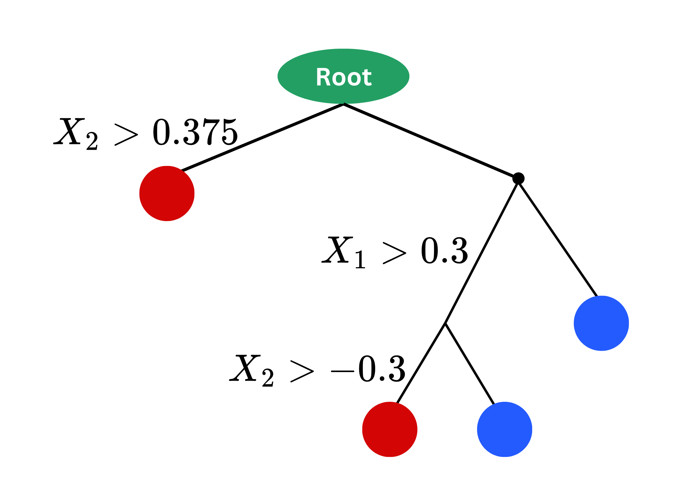
CART: Classification And Regression Trees

• In CART, “neighbors” are defined by rectangular regions within inputs space.

• Neighbors in \(k\)-NN are based on straight distance.

• Neighbors in CART are based on blocks.

🌳 Decision Trees

CART: Classification And Regression Trees

• Building a CART consists of:
  • Start at root (no split yet).
  • Recursively split into smaller regions.
  • Stop when a stopping criterion is met.
• Regions \(\color{blue}{\Rightarrow}\) neighbors \(\color{blue}{\Rightarrow}\) prediction.

• At each split,
  • We try column \(\color{red}{X_j}\) at threshold \(\color{red}{a}\in\mathbb{R}\) into two subregions \(R_1\) and \(R_2\).
  • We decision to split along \(\color{red}{X_j}\) at \(\color{red}{a}\) so that \(R_1\) and \(R_2\) are as pure as possible.
• Impurity is defined by impurity measures:
  • Regression: Within-region variation \(\sum_{y\in R_1}(y-\overline{y}_1)^2+\sum_{y\in R_2}(y-\overline{y}_2)^2.\)
  • Classification (\(M\) classes):
    • Missclassification error \(=1-\hat{p}_{k^*}\) where \(k^*\) is the majority class.
    • Gini impurity \(=\sum_{k=1}^M\hat{p}_{k}(1-\hat{p}_{k})\).
    • Entropy \(=-\sum_{k}\hat{p}_{k}\log(\hat{p}_{k})\) where \(\hat{p}_{k}\): proportion of class \(k\) in region \(R\).

🌳 Decision Trees

CART: Classification And Regression Trees

• Building a CART consists of:
  • Start at root (no split yet).
  • Recursively split into smaller regions.
  • Stop when a stopping criterion is met.
• Regions \(\color{blue}{\Rightarrow}\) neighbors \(\color{blue}{\Rightarrow}\) prediction.

• At each split,
  • We try column \(\color{red}{X_j}\) at threshold \(\color{red}{a}\in\mathbb{R}\) into two subregions \(R_1\) and \(R_2\).
  • We decision to split along \(\color{red}{X_j}\) at \(\color{red}{a}\) so that \(R_1\) and \(R_2\) are as pure as possible.
• Impurity is defined by impurity measures:

The smaller \(\Leftrightarrow\) the purer the regions!

🌳 Decision Trees

CART: Classification And Regression Trees

• First split:
  • \(\text{En}(R_1)=-1\log(1)=0\)
  • \(\begin{align*}\\ \text{En}(R_2)&=-\color{blue}{16/19\log(16/19)}-\color{red}{3/19\log(3/19)}\\ &=0.436.\end{align*}\)
  • \(\text{En}_1=(0)11/30+(0.436)19/30=0.276.\)
  • Information gain: \(\text{En}_0-\text{En}_1.\)

• Prediction rule:
  • Regression: \(\color{blue}{\hat{y}}=\) average targets within the same block.
  • Classification: \(\color{blue}{\hat{y}}=\) majority vote among points within the same block.

🌳 Decision Trees

Hyperparameters of CART and Influence

• Hyperparameters:
  • max_depth
  • max_features
  • min_samples_split
  • min_samples_leaf
  • criterion… [see explanation here]

• Deep trees \(\Leftrightarrow\) less neighbors \(\Rightarrow\) Overfitting.
• In this case of smaller leaves, it’s similar to smaller \(k\) in \(k\)-NN.
• These hyperparameters should be fine-tuned using CV to optimize its performance.

🌳 Decision Trees

In action: Heart Disease Dataset

• We drop duplicated data and use GridsearchCV with \(K=10\) to search over the hyperparameters:
  • Impurity (criterion)
  • Mininum size of leave nodes (min_samples_leaf)
  • Maximum features (max_features).

data = pd.read_csv(path + "/heart.csv")
quan_vars = ['age','trestbps','chol','thalach','oldpeak']
qual_vars = ['sex','cp','fbs','restecg','exang','slope','ca','thal','target']

# Convert to correct types
for i in quan_vars:
  data[i] = data[i].astype('float')
for i in qual_vars:
  data[i] = data[i].astype('category')

# Train test split
from sklearn.model_selection import train_test_split
data_no_dup = data.drop_duplicates()
X, y = data_no_dup.iloc[:,:-1], data_no_dup.iloc[:,-1]
X_train, X_test, y_train, y_test = train_test_split(X, y, test_size=0.2, stratify=y, random_state=42)

from sklearn.model_selection import GridSearchCV 
from sklearn.tree import DecisionTreeClassifier 
from sklearn.metrics import accuracy_score
from sklearn.metrics import roc_auc_score, accuracy_score, precision_score, recall_score, f1_score, confusion_matrix, ConfusionMatrixDisplay

clf = DecisionTreeClassifier()
param_grid = {'criterion': ['gini', 'entropy'],
              'min_samples_leaf': [2, 5, 10, 16, 20, 25, 30],
              'max_features': ['auto', 'sqrt', 'log2', 2, 5, 10, X_train.shape[1]] }
grid_search = GridSearchCV(estimator=clf, param_grid=param_grid, cv=10, scoring='accuracy', n_jobs=-1) 
grid_search.fit(X_train, y_train)

best_model = grid_search.best_estimator_ 
y_pred = best_model.predict(X_test)

test_tr = pd.DataFrame(
    data={'Accuracy': accuracy_score(y_test, y_pred),
          'Precision': precision_score(y_test, y_pred),
          'Recall': recall_score(y_test, y_pred),
          'F1-score': f1_score(y_test, y_pred)},
    columns=["Accuracy", "Precision", "Recall", "F1-score"],
    index=["Tree"])
test_tr = pd.concat([test_tr, pd.DataFrame(
    data={'Accuracy': 0.885246,
          'Precision': 0.882353,
          'Recall': 0.909091,
          'F1-score': 0.909091},
    columns=["Accuracy", "Precision", "Recall", "F1-score"],
    index=["16-NN"])], axis=0)
print(f"Best hyperparameters: {grid_search.best_params_}")
test_tr

Best hyperparameters: {'criterion': 'gini', 'max_features': 10, 'min_samples_leaf': 5}

	Accuracy	Precision	Recall	F1-score
Tree	0.737705	0.742857	0.787879	0.764706
16-NN	0.885246	0.882353	0.909091	0.909091

🌳 Decision Trees

Summary

• CART is a nonparametric model that define neighbors based on small rectangular regions.

• They are not sensitive to scaling.
• The key parameters includes
  • depth, minimum leave size,
  • impurity measures, number of splits,
  • maximum features considered at each split…
• They should be fine-tuned to optimize the model performance.
• It can handle categorical data as well.
• Just ike \(K\)-NN with small \(K\), deep trees are prone to overfitting.

🥳 Yeahhhh….

Let’s Party… 🥂