import pandas as pd # Import pandas packageimport numpy as npimport seaborn as sns # Package for beautiful graphsimport matplotlib.pyplot as plt # Graph managementsns.set(style="whitegrid") # Set grid data = pd.read_csv(path2 +"auto-mpg.csv") # Import it into Pythondata.head(4) # Randomly select 4 points
mpg
cylinders
displacement
horsepower
weight
acceleration
model year
origin
car name
0
18.0
8
307.0
130
3504
12.0
70
1
chevrolet chevelle malibu
1
15.0
8
350.0
165
3693
11.5
70
1
buick skylark 320
2
18.0
8
318.0
150
3436
11.0
70
1
plymouth satellite
3
16.0
8
304.0
150
3433
12.0
70
1
amc rebel sst
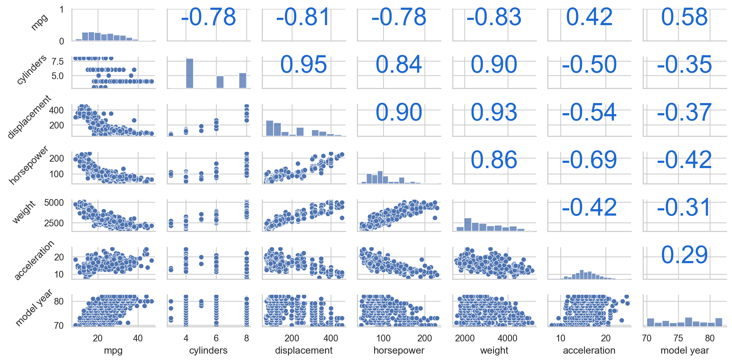
What factors affect fuel efficiency the most?
How much can we predict fuel efficiency of the cars using their characteristics?
Weight shows the strongest negative correlation with mpg, followed by displacement, cylinders, and horsepower. These variables are significant in explaining variations in mpg.
These features are also highly correlated with each other, suggesting potential redundancy when included together in a predictive model.
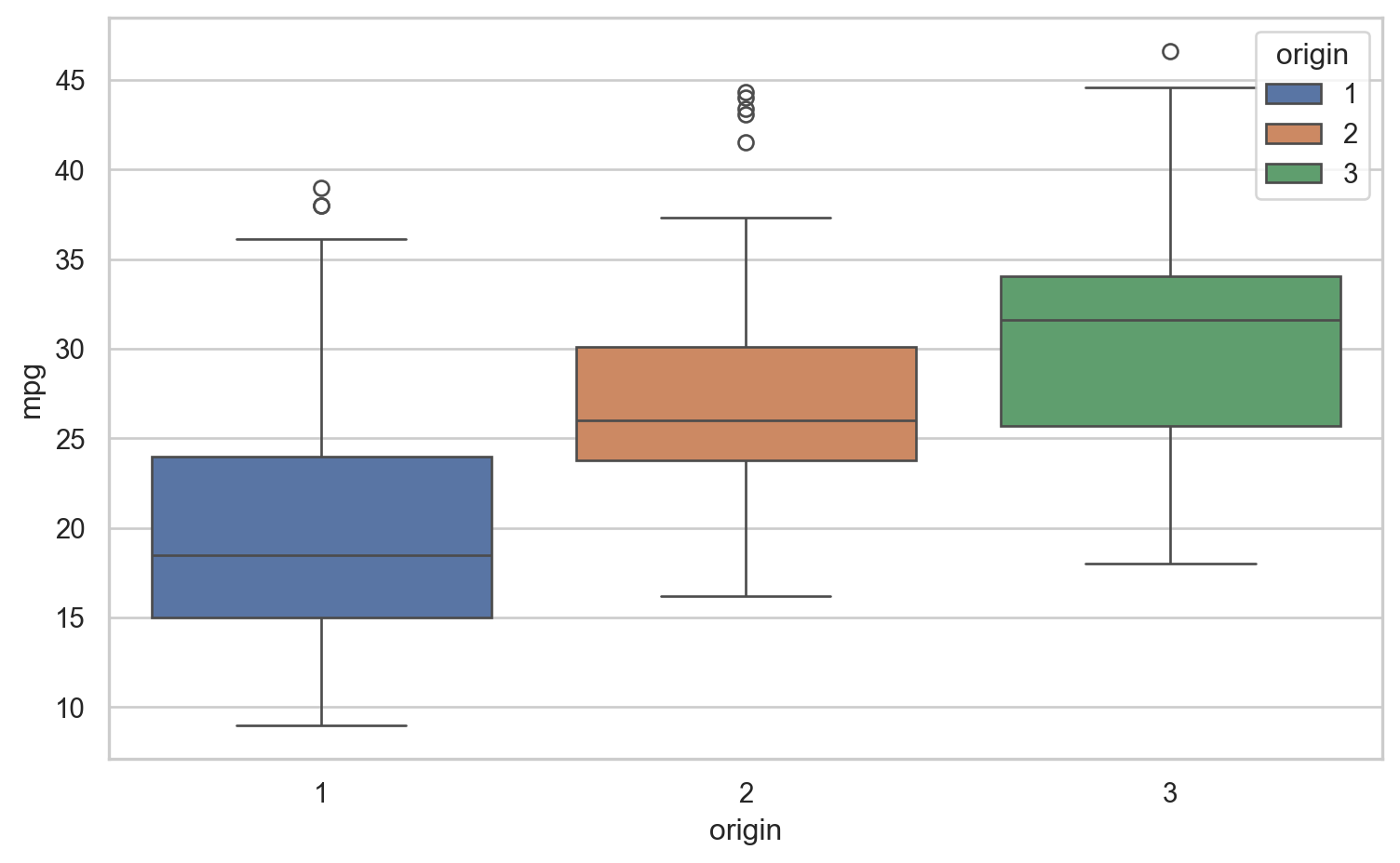
Despite being a categorical variable, origin proves to be valuable for predicting mpg.
Simple Linear Regression (SLR)
Simple Linear Regression (SLR)
mpg vs weight
Code
data[['mpg', 'weight']].head(3)
mpg
weight
0
18.0
3504
1
15.0
3693
2
18.0
3436
Code
import plotly.express as pxfig = px.scatter(data, x="weight", y="mpg", hover_name="car name")fig.update_layout(title="mpg vs weight", height=290, width=450)fig.show()
Simple Linear Model:\[\text{(prediction)}:\quad\widehat{\text{mpg}}_i=\color{blue}{a}\text{weight}_i+\color{blue}{b},\] for some \(\color{blue}{a},\color{blue}{b}\in\mathbb{R}\) to be chosen so that \(\color{red}{\widehat{\text{mpg}}_i\approx \text{mpg}_i}\) for all \(i=1,...,n.\)
In general, \(\hat{y}_i=\color{blue}{a}\text{x}_i+\color{blue}{b}\), with keys \(\color{blue}{a},\color{blue}{b}\), and observed data \((y_i,\text{x}_i),i=1,...,n\).
Objective Find the best \(\color{blue}{a}\) and \(\color{blue}{b}\) so that (prediction) \(\color{red}{\hat{y}_i\approx y_i}\) (reality) for all \(i\).
What does \(\color{red}{\hat{y}_i\approx y_i}\) mean?
Simple Linear Regression (SLR)
mpg vs weight
Code
data[['mpg', 'weight']].head(3)
mpg
weight
0
18.0
3504
1
15.0
3693
2
18.0
3436
Code
fig.update_layout(title="Mpg vs weight", height=290, width=450)fig.show()
What does \(\color{red}{\hat{y}_i\approx y_i}\) mean?
Q2: For \(y_0=20.312\), which one is the best prediction among: \(\color{red}{\hat{y}_0=18.2, 21.5}\) and \(\color{red}{19.73}\)?
Residual Sum of Squares (RSS): \[\begin{align*}\color{red}{\text{RSS}=\sum_{i=1}e_i^2}&=\color{red}{\sum_{i=1}^n(y_i-\color{blue}{\hat{y}_i})^2}\\ &=\color{red}{\sum_{i=1}^n(y_i}-\color{blue}{a}\text{x}_i-\color{blue}{b}\color{red}{)^2}.\end{align*}\]
Roughly, \(\color{red}{\text{RSS}}\) is sum of all the dash lines (squared).
Objective: Find the coefficient \((\color{blue}{a,b})\) that produces smallest \(\color{red}{\text{RSS}}\).
\(\overline{\text{x}}_n=\frac{1}{n}\sum_{i=1}^n\text{x}_i\) and \(\overline{y}_n=\frac{1}{n}\sum_{i=1}^ny_i\): the average/mean of \(X\) and \(Y\) respectively.
\(\text{Cov}(X,Y)=\frac{1}{n}\sum_{i=1}^n(\text{x}_i-\overline{\text{x}}_n)(y_i-\overline{y}_n)\): the “covariance” between \(X\) & \(Y\).
\(\text{V}(X)=\frac{1}{n}\sum_{i=1}^n(\text{x}_i-\overline{\text{x}}_n)^2\): the “variance” of \(X\).
Interpretation: The model (weight) can explain around 69.3% of the variation of the target (mpg).
Simple Linear Regression (SLR)
Model Diagnostics (judging the model)
Residual Analysis
Residuals: If \(\color{red}{e_i=y_i-\hat{y}_i}\sim{\cal N}(0,\sigma^2)\) for some \(\sigma>0\) .i.e., Symmetric around\(0\) & DO NOT DEPEND ON\(\text{x}_i\) nor \(y_i\).
The estimated coefficient \(\color{blue}{\hat{a}}\) and \(\color{blue}{\hat{b}}\) are computed based on a sample of data.
How can we be sure that the linear relation between \(\text{x}\) and \(y\) truely exists: \(\hat{y}=\color{blue}{\hat{a}}\text{x}+\color{blue}{\hat{b}}\) with \(a\neq 0\)?
This is equivalent to testing \(H_0: \color{blue}{\hat{a}}=0\) against \(H_1: \color{blue}{\hat{a}}\neq 0\).
If \(n\) is large enough (\(n>30\)) or the residual is gaussian then if \(H_0\) is true, we have \(\color{blue}{t}=\frac{\color{blue}{\hat{a}}}{s_{\color{blue}{\hat{a}}}}\sim{\cal T}(n-2)\) where \(s_{\color{blue}{\hat{a}}}\) is the standard deviation of \(\color{blue}{\hat{a}}\).
Given \(0\leq\color{red}{\alpha}\leq 1\), let \(\color{red}{t_{\alpha/2}}\) be the \(\color{red}{\alpha}\)-quantile of t-distribution \(\mathbb{P}(|{\cal T}(n-2)|\geq \color{red}{t_{\alpha/2}})=\color{red}{\alpha}\):
We can reject\(H_0\) if \(\color{blue}{t}\geq \color{red}{t_{\alpha/2}}\) (linear relation between \(\text{x}\) & \(y\) truely exists) at confidence level \(1-\color{red}{\alpha}\).
Else, we cannot reject\(H_0\) (not enough evidence to support a linear relationship between \(y\) & \(\text{x}\)).
Simple Linear Regression (SLR)
\(t\)-test for Coefficient
import statsmodels.api as smmodel = sm.OLS(data['mpg'], sm.add_constant(data[['weight']]))results = model.fit()print(results.summary())
                            OLS Regression Results
==============================================================================
Dep. Variable:                    mpg   R-squared:                       0.693
Model:                            OLS   Adj. R-squared:                  0.692
Method:                 Least Squares   F-statistic:                     878.8
Date:                Mon, 08 Sep 2025   Prob (F-statistic):          6.02e-102
Time:                        22:14:42   Log-Likelihood:                -1130.0
No. Observations:                 392   AIC:                             2264.
Df Residuals:                     390   BIC:                             2272.
Df Model:                           1
Covariance Type:            nonrobust
==============================================================================
                 coef    std err          t      P>|t|      [0.025      0.975]
------------------------------------------------------------------------------
const         46.2165      0.799     57.867      0.000      44.646      47.787
weight        -0.0076      0.000    -29.645      0.000      -0.008      -0.007
==============================================================================
Omnibus:                       41.682   Durbin-Watson:                   0.808
Prob(Omnibus):                  0.000   Jarque-Bera (JB):               60.039
Skew:                           0.727   Prob(JB):                     9.18e-14
Kurtosis:                       4.251   Cond. No.                     1.13e+04
==============================================================================

Notes:
[1] Standard Errors assume that the covariance matrix of the errors is correctly specified.
[2] The condition number is large, 1.13e+04. This might indicate that there are
strong multicollinearity or other numerical problems.
As we already rejected\(H_0:\color{blue}{\hat{a}}=0\), the coefficient \(\color{blue}{\hat{a}}=\) -0.008 can be interpreted as follows: mpg is expected to decrease (or increase) by 0.008 units for every \(1\) unit increase (or increase) in car weight.
R-squared: Represents the proportion of the target’s variation (mpg) captured by the model or explanatory variable weight alone.
Residual: In a good model, the residuals should behave like random noise, indicating that the model has captured most of the information/pattern from the target.
Our example:
The weight of cars alone can explain \(\approx 70\)% (R-squared) of the variation of mpg.
However, the residuals still contain patterns (large errors at large predicted mpg), suggesting the model can be improved.
Multiple Linear Regression (MLR)
Multiple Linear Regression (MLR)
mpg vs cylinders + year
Multiple Linear Regression:using more than 1 input, for example: \[\begin{align*}\widehat{\text{mpg}}_i&=\color{blue}{\beta_0} + \color{blue}{\beta_1}\text{acc}_i+\color{blue}{\beta_2}\text{year}_i\\(\text{Maths:}\quad \hat{y}_i&=\color{blue}{\beta_0} + \color{blue}{\beta_1}\text{x}_{i1}+\color{blue}{\beta_2}\text{x}_{i2}),\end{align*}\] with \(\color{blue}{\beta_0,\beta_1,\beta_2}\in\mathbb{R}\) to be estimated.
We find \([\color{blue}{\hat{\beta}_0,\hat{\beta}_1,\hat{\beta}_2}]\) minimizing \[\begin{align*}\color{red}{\text{RSS}}&=\sum_{i=1}^n(y_i-\color{blue}{\hat{y}_i})^2\\ &=\sum_{i=1}^n(y_i-\color{blue}{\beta_0}-\color{blue}{\beta_1}\text{x}_{i1}-\color{blue}{\beta_2}\text{x}_{i2})^2.\end{align*}\]
Normally, \(R^2\) increases along with the number of inputs, but a good model may not need so many variables.
A better criterion, Adjusted R-squared (balancing the number of inputs with the increment in\(R^2\)): \[R^2_{\text{adj}}=1-\frac{n-1}{n-d-1}(1-R^2).\] Here, \(n\) is the number of observations, \(d\) is the number of inputs.
Usually, \(R^2_{\text{adj}}\leq R^2\).
For our model: \(R^2=\) 0.715 and \(R^2_{\text{adj}}=\) 0.714 (this is a good sign!).
A large \(R^2\) with a slight drop in \(R^2_{\text{adj}}\) indicates a good MLR model.
Rough interpretion, \(\beta_1=\) -2.998 indicates that if cylindersincrease (or decreases) by \(1\) unit, mpg is expected to decrease (or increase) by 2.998 units.
Explain: \(\beta_2=\) 0.75.
\(R^2=\) 0.715 indicates that around 71.5% variation of mpg can be explained by cylinders and year together, which is better than weight alone.
A slight decrease in \(R^2_{\text{adj}}=\) 0.714 suggests that the information provided by both variables is not redundant for explaining mpg.
The spread values of residuals around large predicted mpg indicates that the model underestimates the actual target.