🗺️ Content
Motivation & Introducion
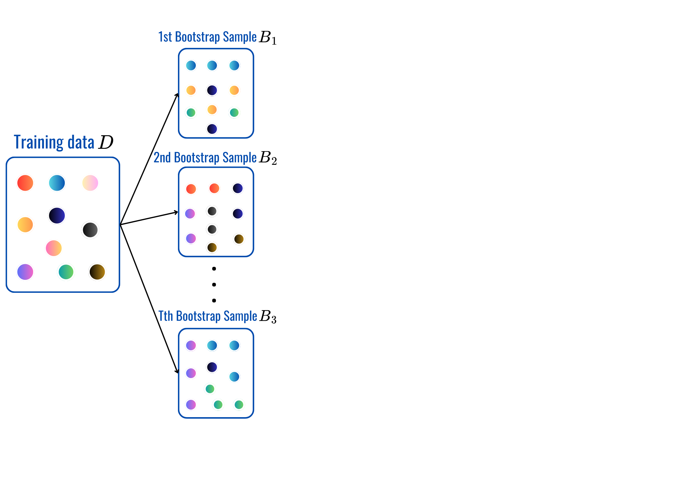
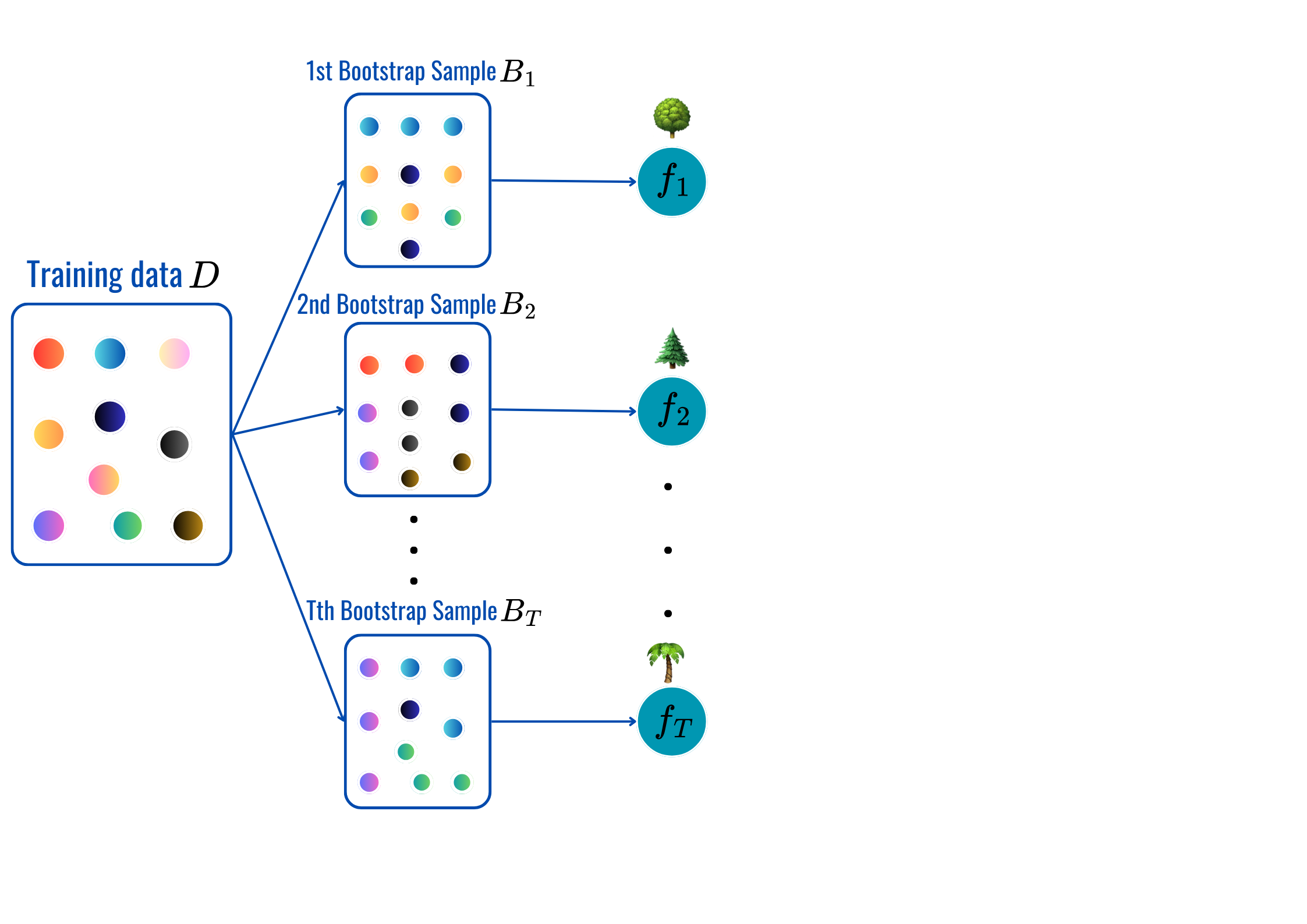
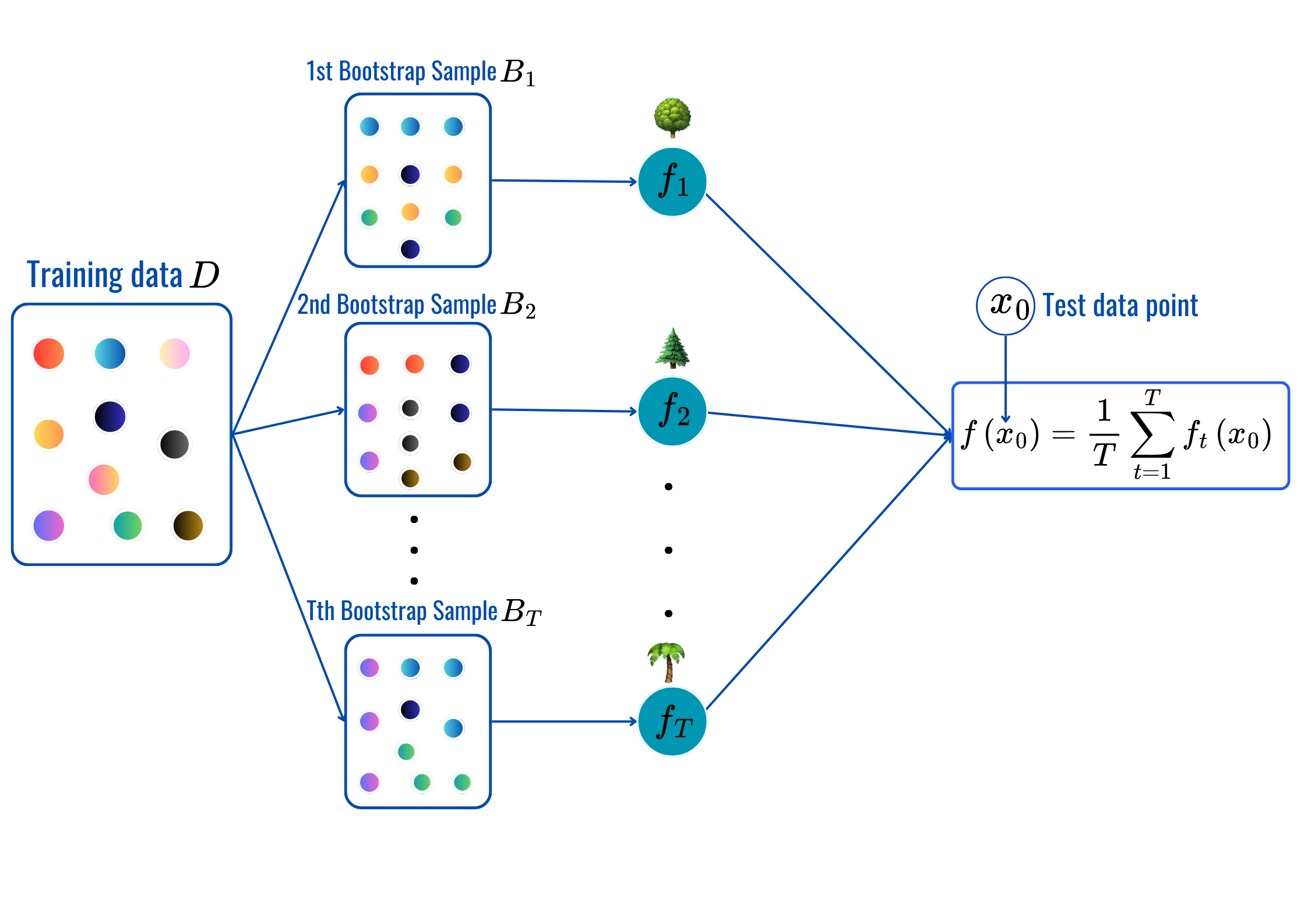
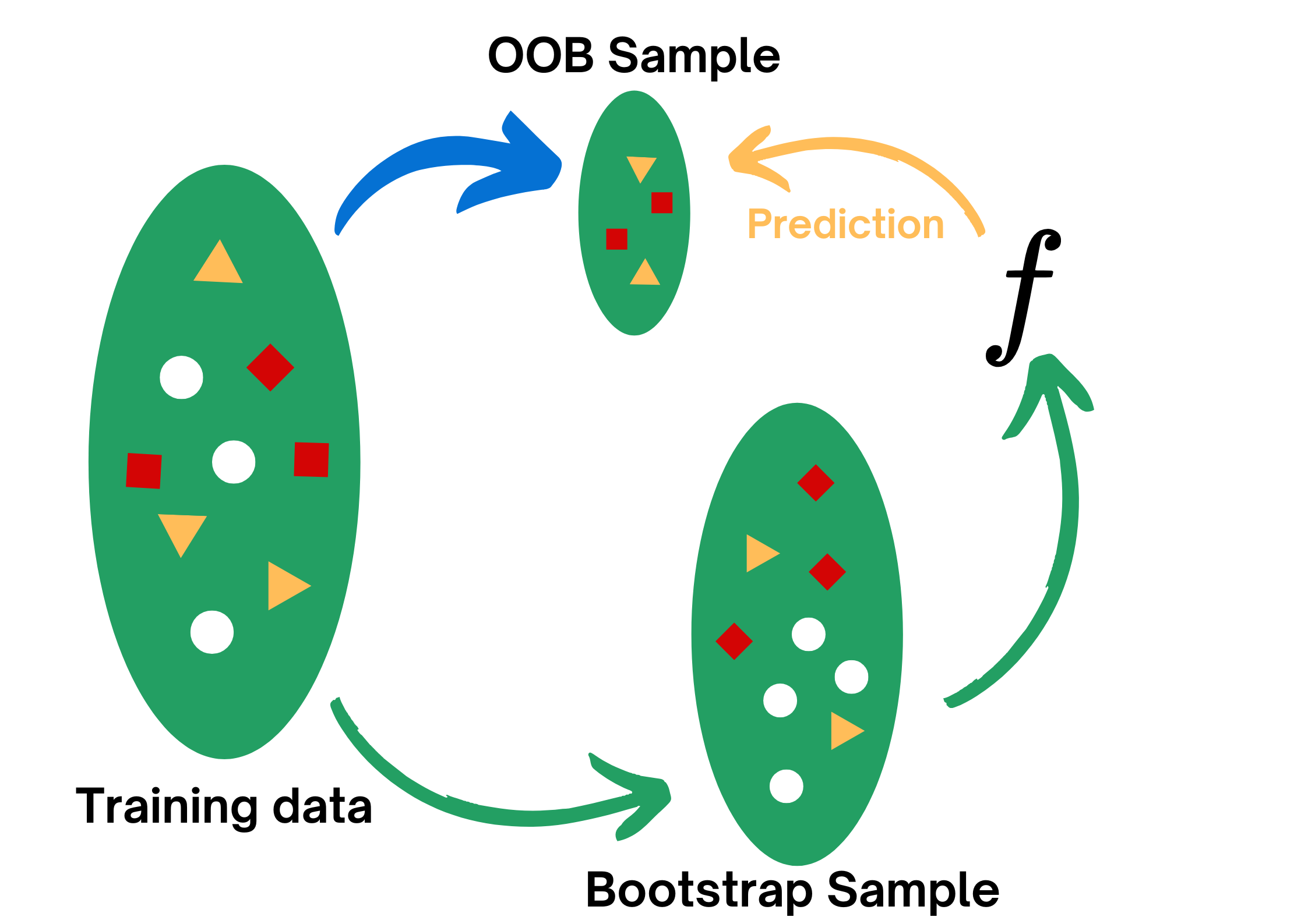
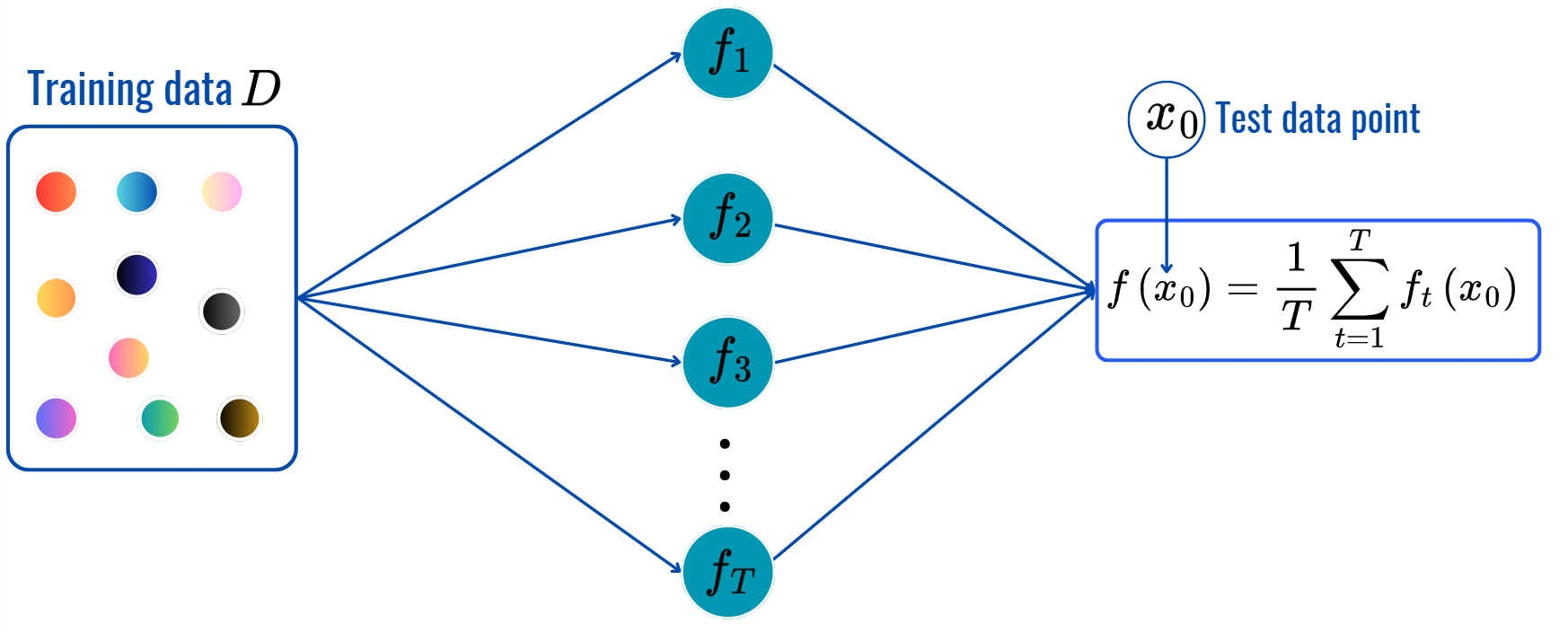
Bootstrap Aggregating: Bagging
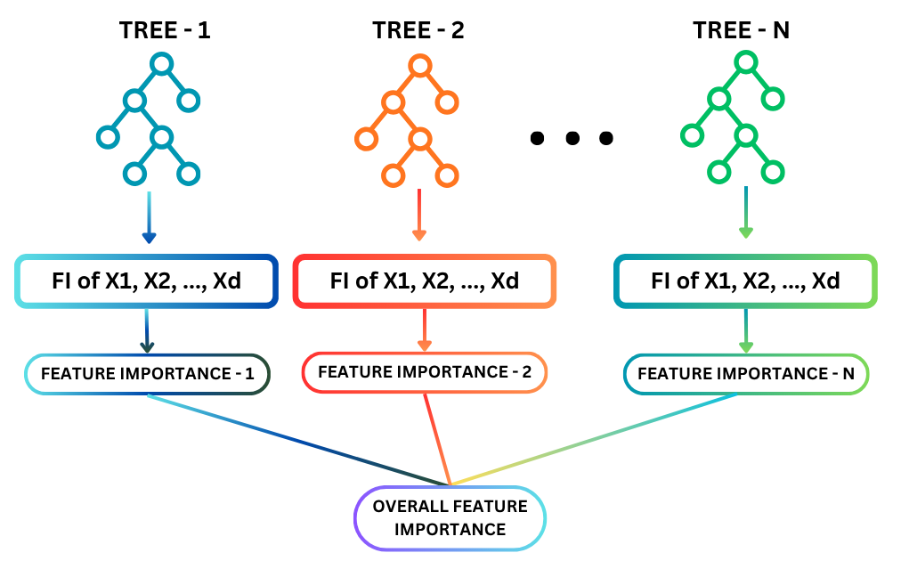
Random Forest
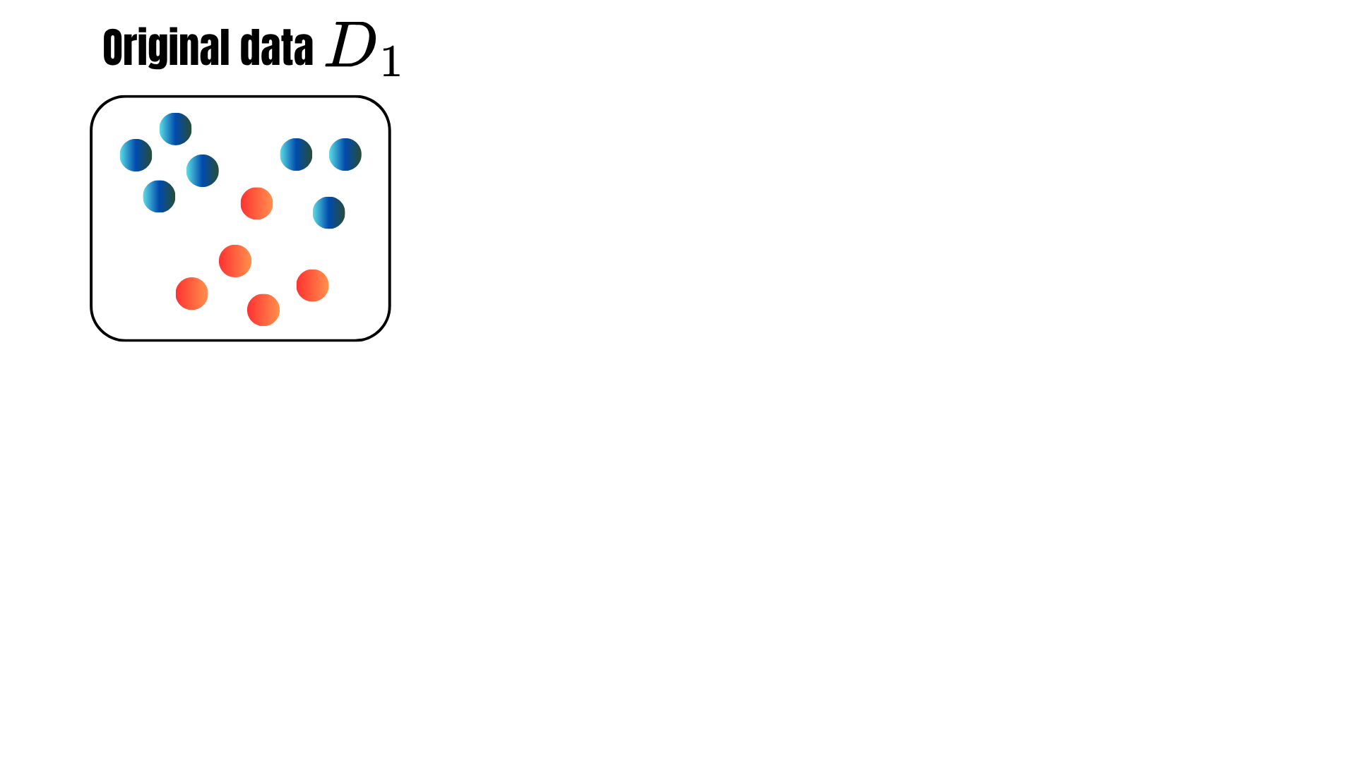
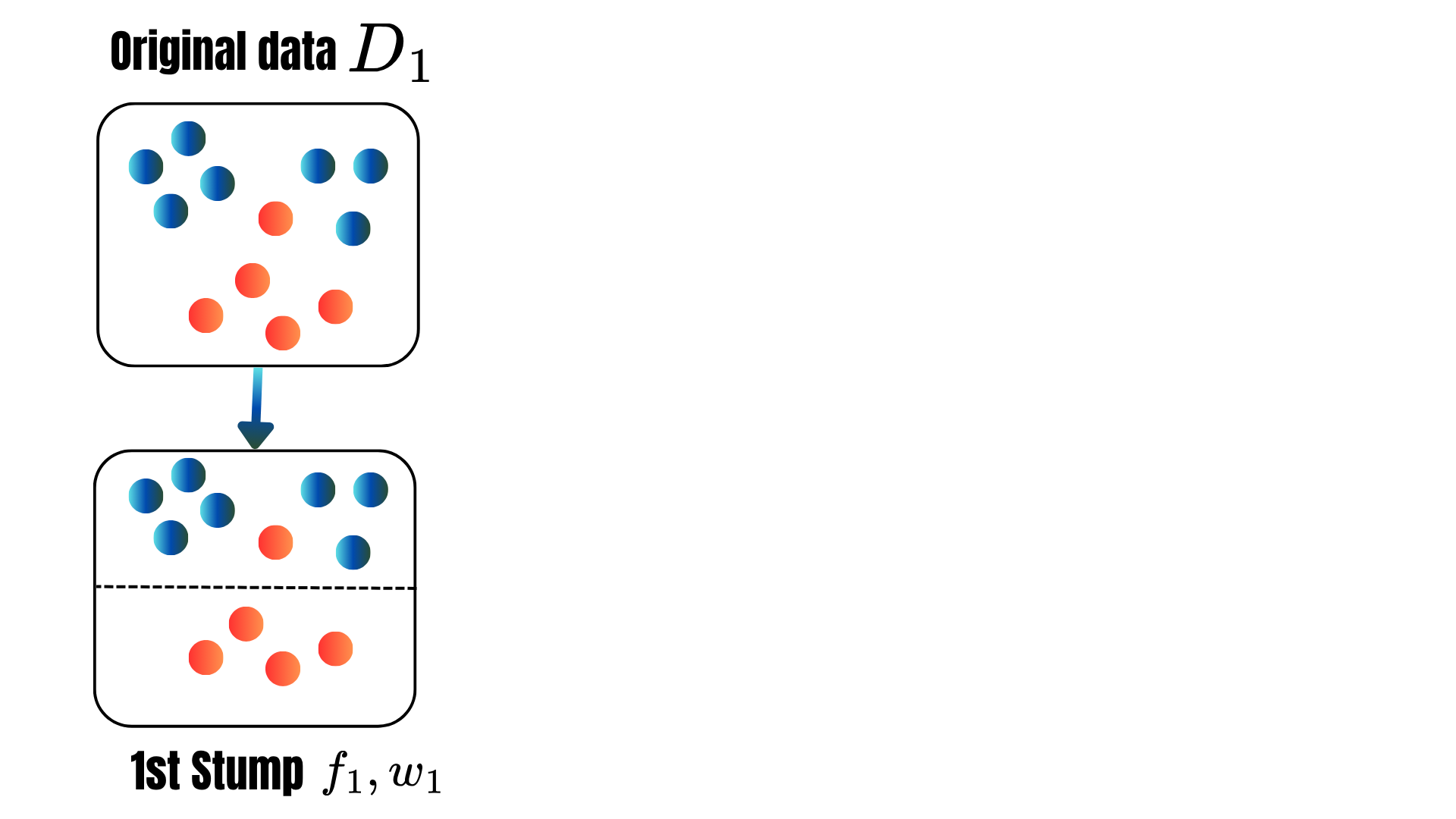
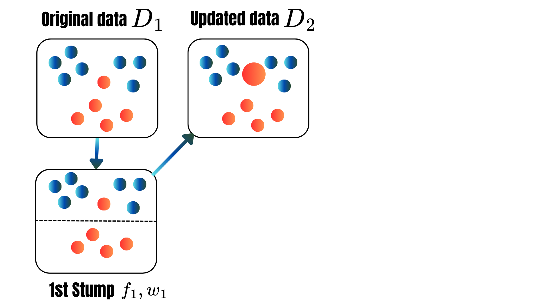
Boosting: Adaboost & XGBoost
Concensual aggregation: Gradient COBRA
ITM 390 004: Machine Learning
![]()
Why do we trust a panel of judges more than a single judge in competitions?
In medicine, why do doctors often seek second or third opinions for complex cases?
Have you noticed that weather forecasts often give a probability of rain rather than a simple yes/no prediction?
Would the famous “Wisdom of Crowds” principle applies to machine learning?
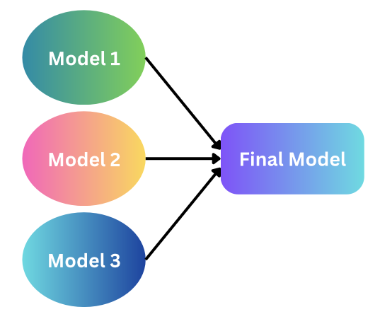
The keys idea of ensemble learning is combining multiple base models/learners to create a better/stronger one.
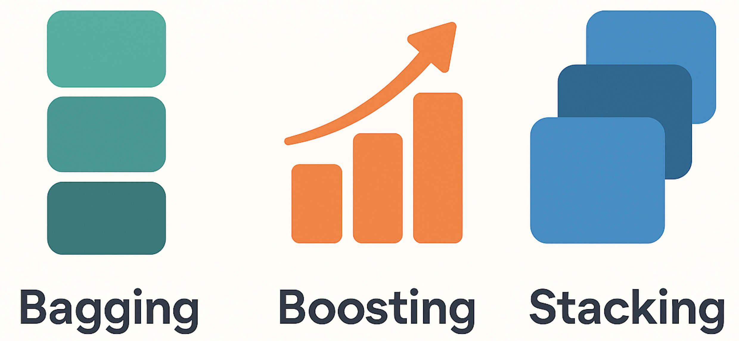
Bagging: Combine nearly decorrelated high-varianced models.
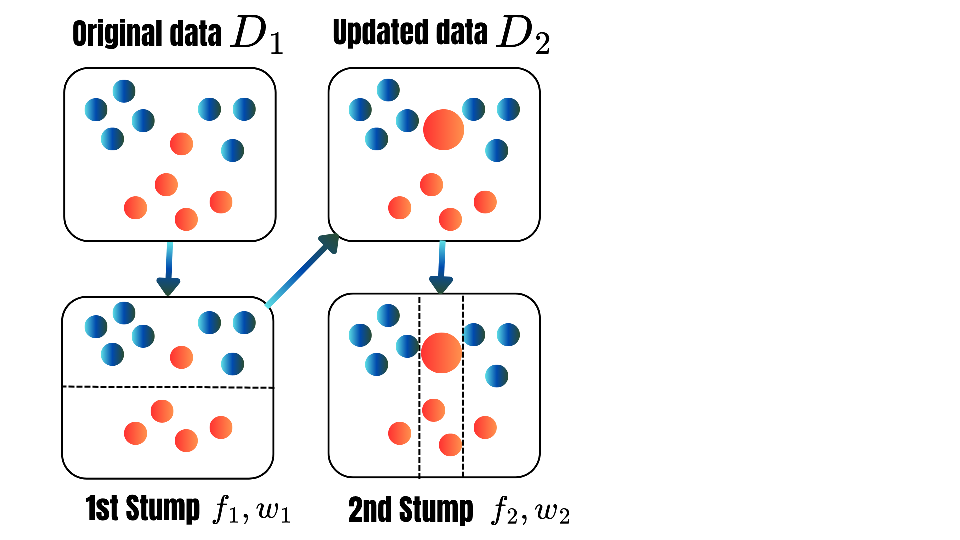
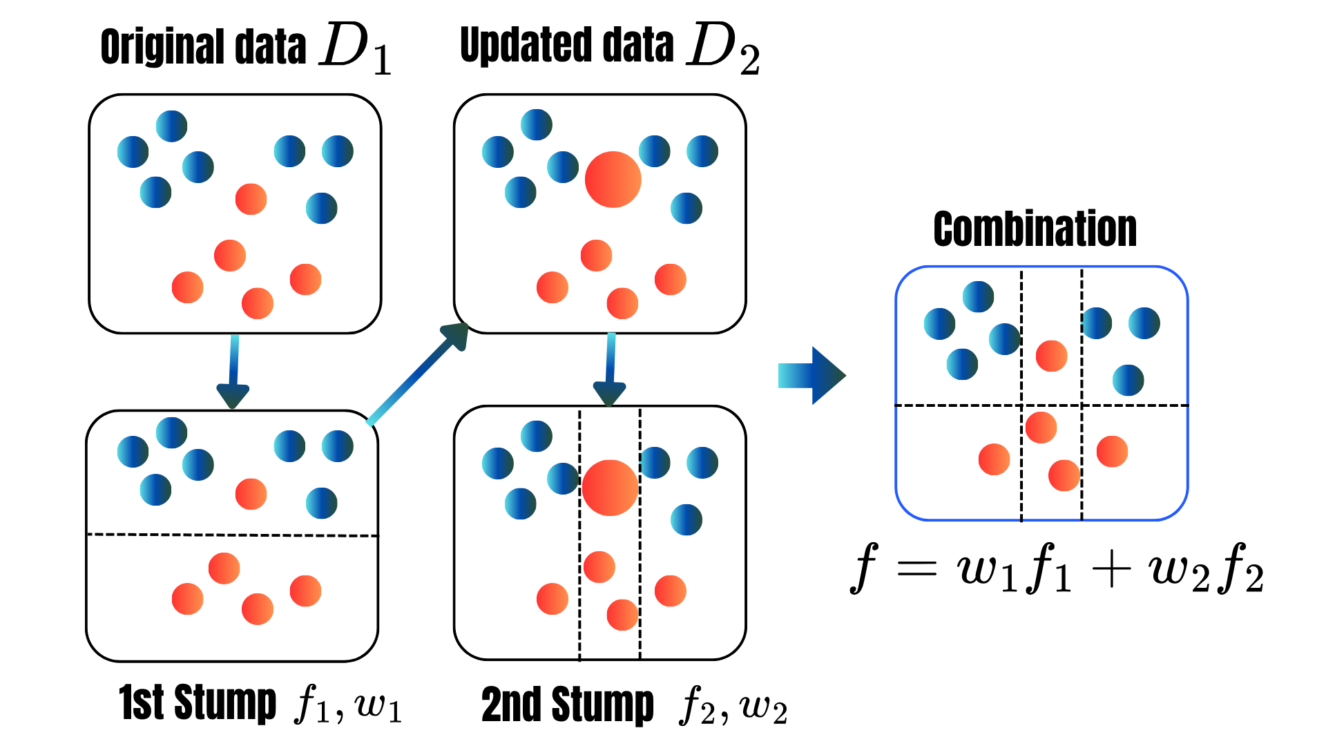
Boosting: Sequentially combine weak learners to create a strong final model.
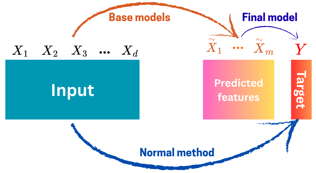
Stacking: Combination is based on the predicted features.
for t = 1,2,...,T:
Prediction: (same as before).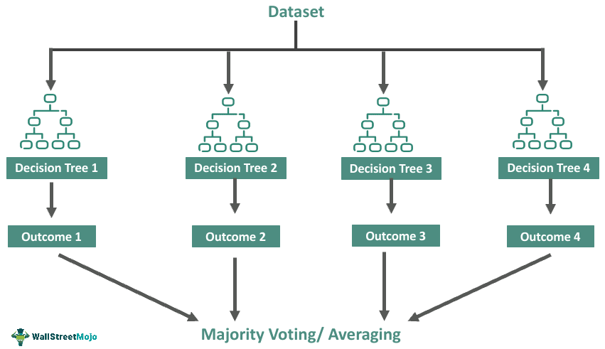
for t = 1,2,...,T:
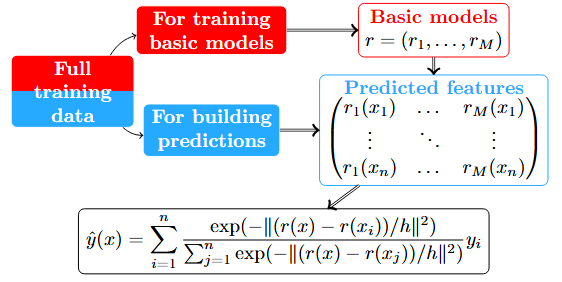
\[\varphi(\color{blue}{h})=\frac{1}{K}\sum_{k=1}^K\sum_{(\text{x}_i,y_i)\in F_j}(\hat{y}_i-y_i)^2.\]
 Gradient Cobra Library