III. Data Quality & Preprocessing

Exploratory Data Analysis & Unsupervised Learning

Lecturer: Dr. HAS Sothea
..Instructor: Ms. UANN Sreyvi

Resources

Applied Missing Data Analysis by Graig K. Enders.

Python for Data Analysis by Wes McKinney, 3rd edition.

1 Data Sources

1.1 Data sources

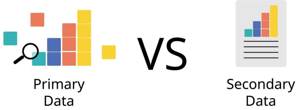
Primary

Data collected directly from the source for a specific purpose.
Example:
- Surveys or Questionnaires 🗳️
- Interviews 🎙️
- Observations 🧐
- Experiments 🔬

Secondary

Data that has already been collected, processed, and made available by others.

Example:
- Government publications or reports 📄
- Books and articles 📚
- Online repositories (Kaggle, Google) 🌐
- Industry/NGO reports 🏭

Format

Structured

Highly organized and easily searchable in databases using predefined schemas.

Format: typically stored in tables with rows and columns.
Example:
- Spreadsheets: Excel
- CSV files

Unstructured

Lacks a predefined format or schema and is typically stored in its raw form.

Format: Free-form and can be text, images, videos…
Example:
- Emails/Documents (e.g., Word files, PDFs) 📄
- Social media posts, images, audio, videos 📷
- Web pages… 🌐

2 Data Quality

2.1 Data quality

Someone in 60s said Garbage In, Garbage Out (GIGO)!.
Data quality is the most important thing in Data Analysis.
Before the analysis, we should always check the quality of our data and make sure that they are good enough for our intended use.
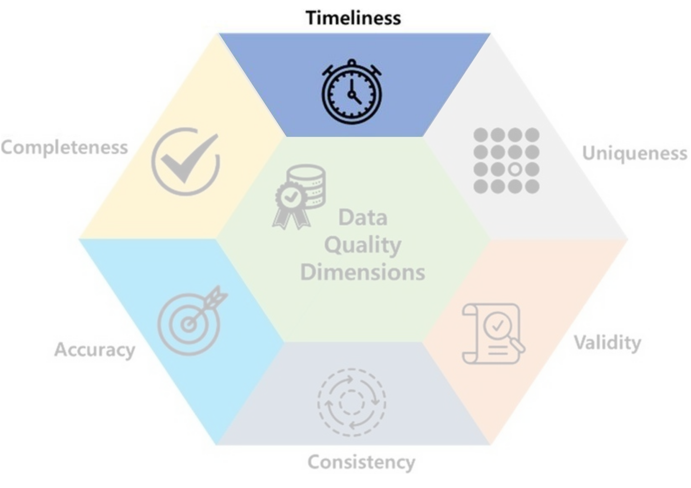
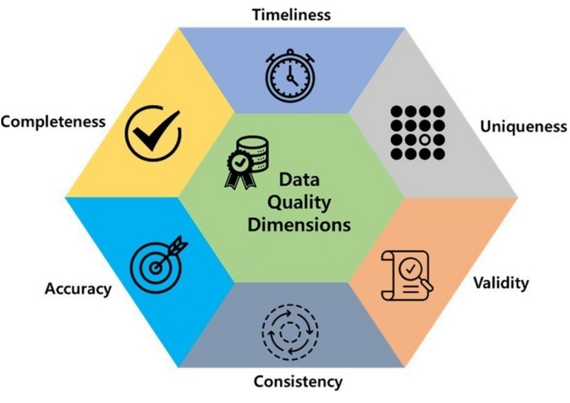
There are several dimensions of data quality to consider. Let’s explore the important ones!

Code

import kagglehub
import plotly.express as px
df_fb = pd.read_csv(path_FB)
fig = px.line(
    df_fb, 
    x="Date", 
    y="Close", 
    title="Facebook Stock Prices Over Time")
df_temp = df_fb.query("Date <= '2013-10-01'")
start_date = df_temp.Date.iloc[0]
end_date = df_temp.Date.iloc[-1]
fig.add_vrect(
    x0=start_date,           
    x1=end_date, 
    fillcolor="red",  
    opacity=0.3,      
    layer="below",   
    line_width=0,
    
)

df_temp = df_fb.query("Date >= '2020-10-01'")
start_date = df_temp.Date.iloc[0]
end_date = df_temp.Date.iloc[-1]
fig.add_vrect(
    x0=start_date,           
    x1=end_date, 
    fillcolor="green",  
    opacity=0.3,      
    layer="below",   
    line_width=0,
    
)
fig.update_layout({
    'paper_bgcolor': 'rgba(0,0,0,0)',
    'plot_bgcolor': 'rgba(0,0,0,0)'},
    width=400, height=250)
# 2. Add the royal blue frame by mirroring the x and y axes
fig.update_xaxes(
    showline=True, 
    linewidth=1, 
    linecolor='gray', 
    mirror=True,  # Mirrors the bottom x-axis line to the top
    showgrid=True, gridwidth=1, gridcolor=LIGHT_GRAY
)
fig.update_yaxes(
    showline=True, 
    linewidth=1, 
    linecolor='gray', 
    mirror=True,  # Mirrors the left y-axis line to the right
    showgrid=True, gridwidth=1, gridcolor=LIGHT_GRAY
)
fig.show()

Timeliness: up-to-date for its intended use?

Temperature of 60s wouldn’t be helpful for forecasting tomorrow temperature.

Stock prices last year wouldn’t be useful now.

	Survived	Embarked	Sex
0	0	Q	male
1	1	S	female
2	0	Q	male
3	0	Q	male
4	1	Q	female
5	0	S	male

From Kaggle Titanic dataset.

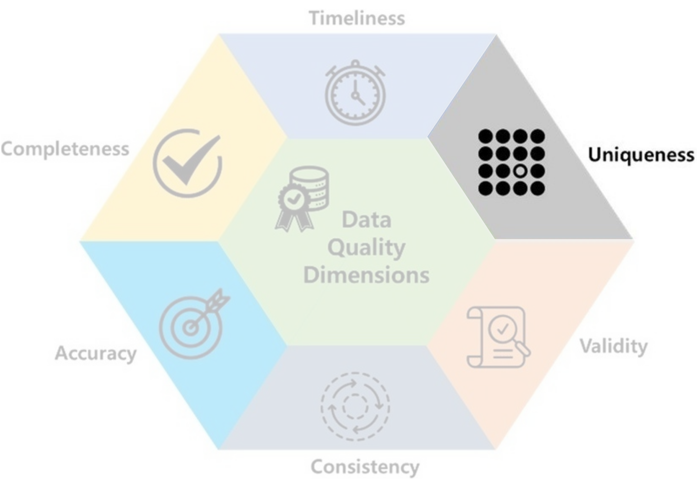
Uniqueness: data shouldn’t be accidentally duplicated.
- Accidentally recording the same patient multiple times may alter the analysis results.
- Predictive models may be biased if the same data point is used for both training and testing.

Code

data_heart = pd.read_csv(path_heart)
fig = px.box(
    data_heart, 
    x="Cholesterol", 
    title="Distribution of Cholesterol Levels",
    points="all")
fig.update_layout({
    'paper_bgcolor': 'rgba(0, 0, 0, 0)',
    'plot_bgcolor': 'rgba(42, 77, 152, 0)'},
    width=400, height=250)
# 2. Add the royal blue frame by mirroring the x and y axes
fig.update_xaxes(
    showline=True, 
    linewidth=1, 
    linecolor='gray', 
    mirror=True,  # Mirrors the bottom x-axis line to the top
    showgrid=True, gridwidth=1, gridcolor=LIGHT_GRAY
)
fig.update_yaxes(
    showline=True, 
    linewidth=1, 
    linecolor='gray', 
    mirror=True,  # Mirrors the left y-axis line to the right
    showgrid=True, gridwidth=1, gridcolor=LIGHT_GRAY
)
fig.show()

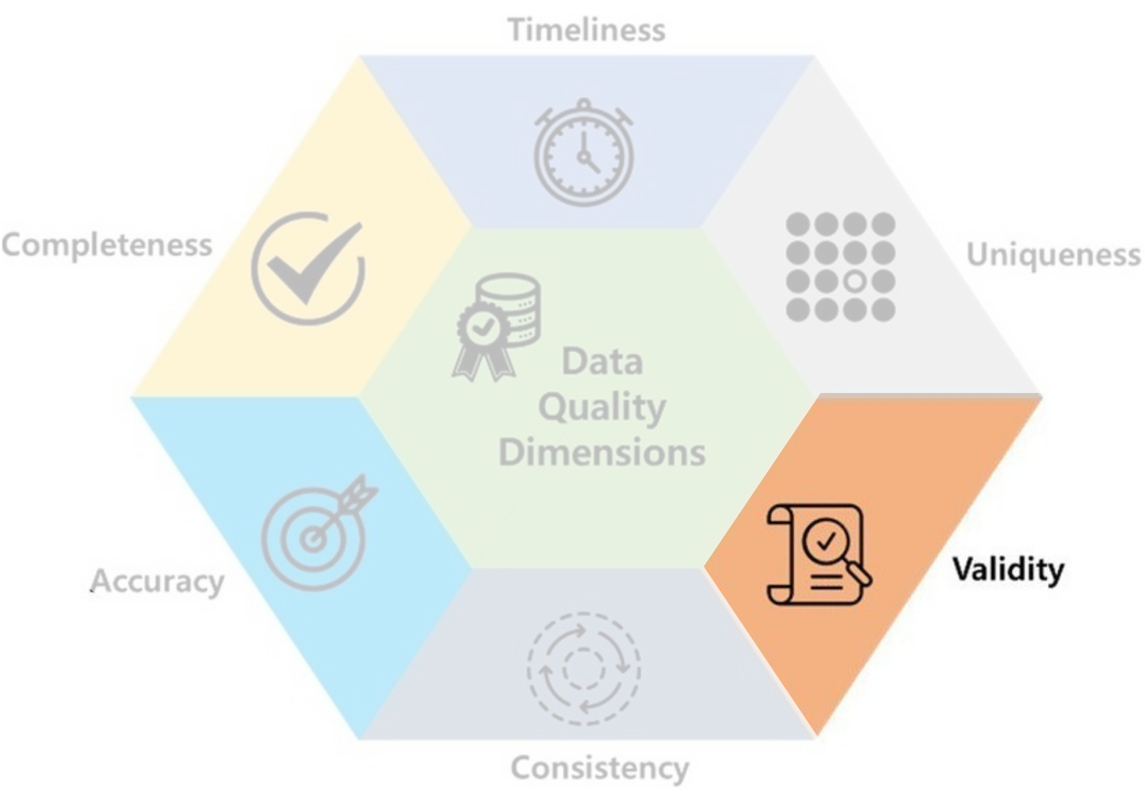
Validity: data should take values within its valid range. Domain knowledge is often required to determine the valid range of values.
- Height & weight should not be 0 nor negative!
- Cholesterol level should not be negative!

	Neck (cm)	Waist (cm)	Height (m)
0	32.0	63.0	160.00
1	13.5	27.0	1.65
2	33.0	67.0	1.65
3	44.7	115.3	176.00
4	35.0	76.0	1.65

Real data from a small survey available here.

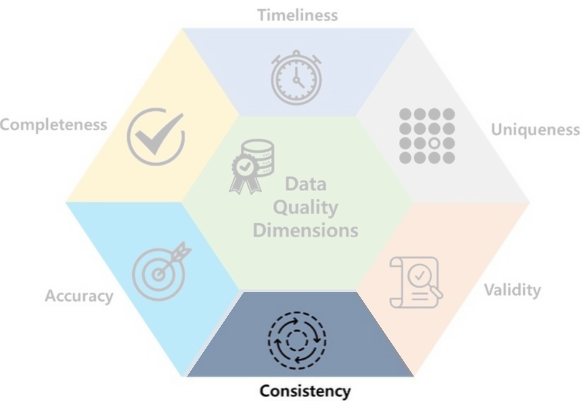
Consistency: data should be uniform and compatible (format, type…) across different datasets and over time.
- Data: 15/03/2004 & 03/15/2004, Gender: Male & M…
Common in secondary sources: data are collected from multiple sources or participants can enter their own data.

	Financial problem	Learning difficulty	Score
0	2	3	90
1	4	5	57
2	7	3	82
3	3	3	55
4	6	6	45

An example of inaccurate data due to confusion.

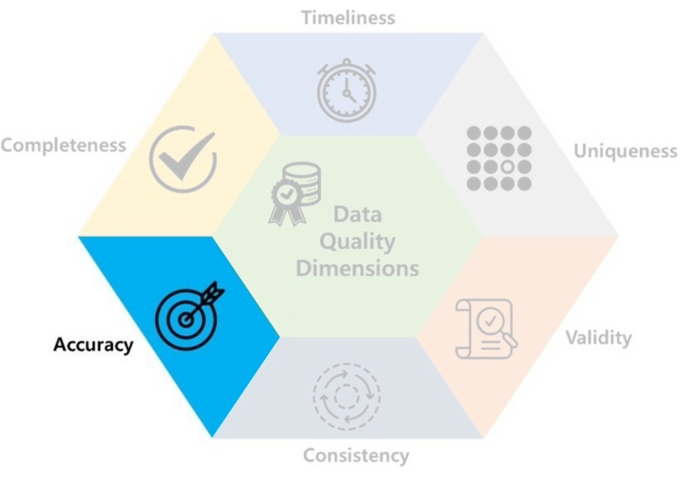
Accuracy: data should be accurate and reflects what it is meant to measure. It’s the hardest to detect!
- You cried and filled ‘I like Data Analysis Course SO MUCH 😭!’ in a non-anonymous survey.

	Sex	Survived	Cabin
0	male	0	NaN
1	female	1	NaN
2	male	0	NaN
3	male	0	NaN
4	female	1	NaN

A subset of Titanic dataset.

Completeness: data shouldn’t contain missing values.
Very often, they are are inevitable and commonly encoded as NaN, nan, NA, null…
Sometimes they may disguish as 0, -1 or other values.

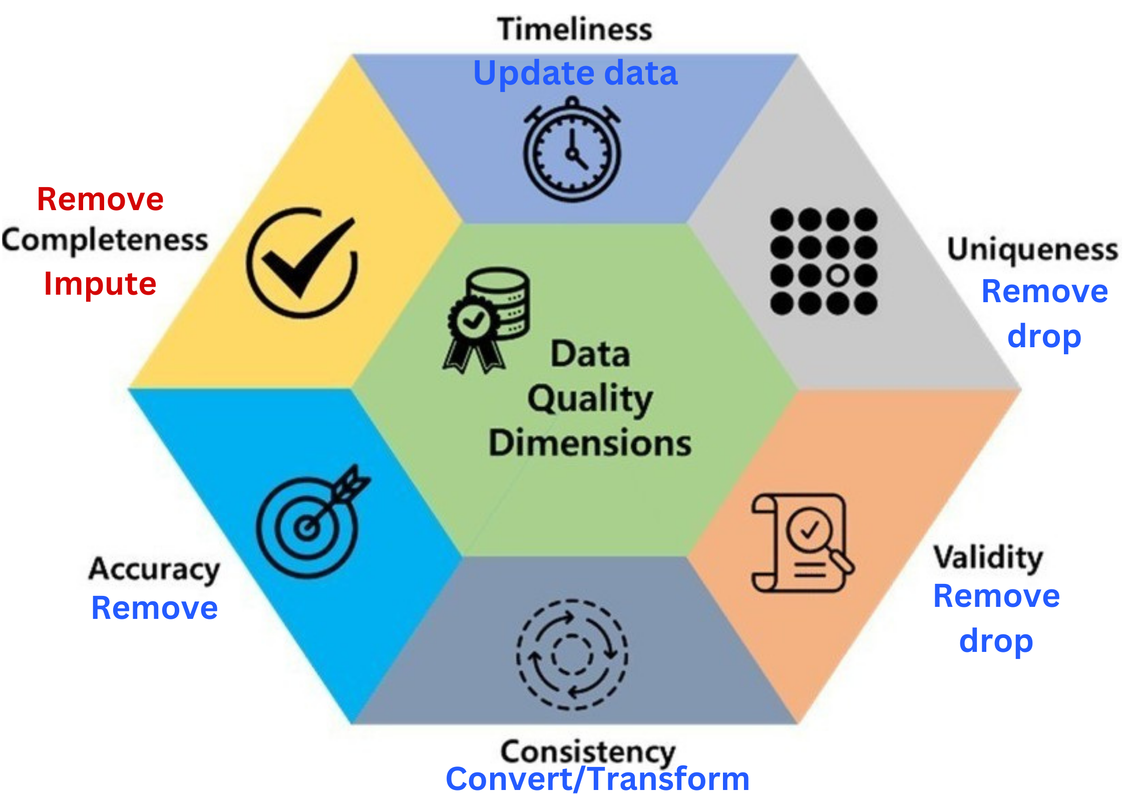
Data quality includes these 6 factors.

Data quality includes these 6 factors.
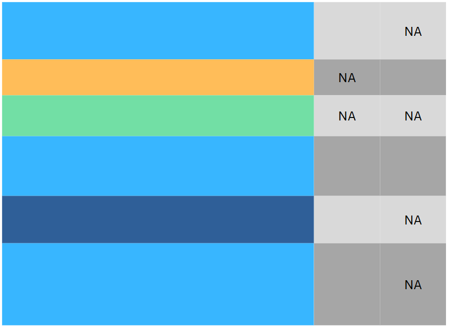
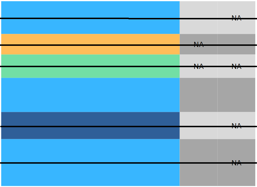
If there is a problem with any of these, you may ☝️

For secondary sources, Incompleteness is the most common one.

3 Data Preprocessing

3.1 Data preprocessing

Drop rows vs drop columns

	Sex	Pclass	Fare	Cabin
0	male	3	7.8292	NaN
1	female	3	7.0000	NaN
2	male	2	9.6875	NaN
3	male	3	8.6625	NaN
4	female	3	12.2875	NaN
5	male	3	9.2250	NaN
6	female	3	7.6292	NaN
7	male	2	29.0000	NaN
8	female	3	7.2292	NaN

	Sex	Pclass	Fare	Cabin
0	male	3	7.8292	NaN
1	female	3	7.0000	NaN
2	male	2	9.6875	NaN
3	male	3	8.6625	NaN
4	female	3	12.2875	NaN
5	male	3	9.2250	NaN
6	female	3	7.6292	NaN
7	male	2	29.0000	NaN
8	female	3	7.2292	NaN

data.dropna(inplace=True)

	Sex	Pclass	Fare	Cabin
0	male	3	7.8292	NaN
1	female	3	7.0000	NaN
2	male	2	9.6875	NaN
3	male	3	8.6625	NaN
4	female	3	12.2875	NaN
5	male	3	9.2250	NaN
6	female	3	7.6292	NaN
7	male	2	29.0000	NaN
8	female	3	7.2292	NaN

data.drop(columns = ['Cabin'])

3.2 Missing values

An example

Data of \(4\)-\(7\) years old kids.

Gender	Age	Height	Weight
F	68	0	20
F	68	0	18
F	65	105	0
F	63	0	15
F	68	112	0

What’s wrong with this data?

These are probably missing values in disguise.
🤔: how do we handle it: Drop or Impute?
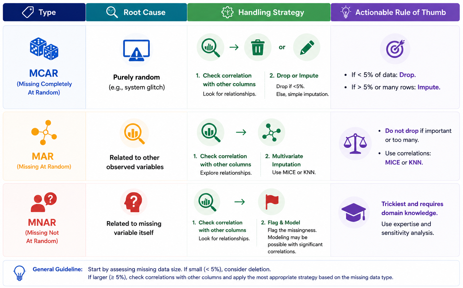
🤓: we should know their types: MCAR, MAR or MNAR?

Missing values (1)

Missing Completely At Random (MCAR)

Gender	Age	Height	Weight
F	63	0	15
M	72	121	25
M	74	116	18
F	68	0	20

Code

import plotly.graph_objects as go
import plotly.express as px
from plotly.subplots import make_subplots
data_dropped_NA = data_kids.loc[(data_kids.Height > 0) & (data_kids.Weight > 0)]
fig_kid1 = go.Figure(go.Histogram(
    x=data_kids.Age, 
    name="Before dropping NA", 
    showlegend=True))
fig_kid1.add_trace(
    go.Histogram(
        x=data_dropped_NA.Age, 
        name="After dropping NA", 
        showlegend=True, 
        visible="legendonly"))
fig_kid1.update_layout(barmode='overlay', 
                       title="Distribution of Age", 
                       xaxis=dict(title="Age"),
                       yaxis=dict(title="Count"),
                       width=400,
                       height=200)
fig_kid1.update_traces(opacity=0.5)
fig_kid1.show()

MCAR: The missingness is completely random and NOT related to its own column nor any other variables.
This implies that dropping them does not affect other columns.
⚠️ Warning: this doesn’t mean the variable itself is not related to other columns, only the missing behavior is random!

Missing values (2)

Missing At Random (MAR)

Gender	Age	Height	Weight
F	63	0	15
M	72	121	25
M	74	116	18
F	68	0	20

Code

count = data_kids.Gender.value_counts()
fig_kid2 = go.Figure(
    go.Bar(
        x=count.index, 
        y=count, 
        name="Before dropping NA"))
count_NA = data_dropped_NA.Gender.value_counts()
fig_kid2.add_trace(
    go.Bar(x=count_NA.index, 
    y=count_NA, 
    name="After dropping NA", 
    visible="legendonly"))
fig_kid2.update_layout(barmode='overlay', 
                       title="Distribution of Gender", 
                       xaxis=dict(title="Gender"),
                       yaxis=dict(title="Count"),
                       width=400,
                       height=200)
fig_kid2.update_traces(opacity=0.5)
fig_kid2.show()

The missingness is NOT related to its own column but related to some other columns within the dataset.
This implies that dropping them will affect other columns.
To handle them, one should consider how the non-missing values of the query column is related to the related to the other columns.

Missing values (3)

Missing Not At Random (MNAR)

These are the trickiest, as the missingness is related to the variable itself and/or maybe other columns.
It’s hard to judge if the missing values are actually MNAR without domain knowledge.
It may require domain-specific knowledge or advanced techniques (more data, external info…).
If not so many, dropping is a common solution.
Ex: Too high or low incomes are often missing…

Handling missing values

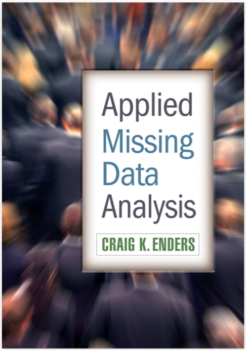
Read, for example, Applied Missing Data Analysis by Graig K. Enders

Rules of Thumb

Prop of `NA`	Rules of thumb 👍
\(< 5\%\)	Drop/remove rows.
\(5-10\%\)	Can be dropped with large sample but must be cautious about the type of missing.
\(10-20\%\)	Better to be imputed according to their types.
\(20-30\%\)	Remove the entire column, if it’s not so important.
\(>30\%\)	Remove the entire column.

3.3 Outliers vs Leverage Points

Univerate outliers

In univariate analysis, outliers are data points that deviate significantly from the majority of observations in a dataset.
We can hunt them down using:
- Graphs: Boxplots or Histograms…
- For normal distribution: around \(99.3\%\) fall within \([\text{Q}_1-1.5\text{IQR},\text{Q}_3+1.5\text{IQR}]\). Therefore, around \(0.7\%\) outside this range are considered outliers.

Code

import scipy.stats as stats
import numpy as np
import plotly.graph_objects as go

# add normal density
y_range = np.linspace(data_dropped_NA.Height.min(), data_dropped_NA.Height.max(), 100)
# Use the mean and standard deviation of your data to fit the normal curve
mu, std = data_dropped_NA.Height.mean(), data_dropped_NA.Height.std()
pdf = stats.norm.pdf(y_range, mu, std)
# Scale the PDF so it fits nicely alongside the boxplot (adjust the multiplier as needed)
scaled_pdf = pdf/pdf.max()

fig_H = go.Figure()

fig_H.add_trace(
    go.Box(
        y=data_dropped_NA.Height,
        name="Height",
        opacity=0.8,
        x0=0, # Places the box exactly at x=0
        marker_color='#1f77b4' # Standard Plotly blue
    )
)
fig_H.add_trace(
    go.Scatter(
        x=scaled_pdf, 
        y=y_range,
        mode='lines',
        name='PDF',
        line=dict(
            color='red', 
            width=2,
            dash='dash')))
fig_H.update_layout(
    {'paper_bgcolor': 'rgba(0, 0, 0, 0)',
    'plot_bgcolor': 'rgba(42, 77, 152, 0)'},
    title="Children's Heights distribution",
    height=370, width=270,
    xaxis=dict(
         title="Height (cm)",
         type='linear',
         range = [-0.5,1.1],
         showticklabels=False))
fig_H.update_xaxes(
    showline=True, 
    linewidth=1,
    linecolor='gray',
    mirror=True, 
    showgrid=True, gridwidth=1, gridcolor=LIGHT_GRAY)
fig_H.update_yaxes(
    showline=True, 
    linewidth=1, 
    linecolor='gray',
    mirror=True,
    showgrid=True, gridwidth=1, gridcolor=LIGHT_GRAY)
fig_H.show()

Bivariate outliers & high leverage points

Outliers should be detected in Univariate Analysis step because it might cause problems in later Multivariate Analysis.

Code

data_abalone = pd.read_csv(path_abalone)
colors = ['Normal' if x < 0.4 else 'Extreme' for x in data_abalone['Height'].values]
fig_outlier = px.scatter(
    data_abalone,
    x="Height",
    y="Rings",
    opacity=0.5,
    color=colors,
    size = [7] * data_abalone.shape[0])
fig_outlier.update_layout(
    {'paper_bgcolor': 'rgba(0, 0, 0, 0)',
    'plot_bgcolor': 'rgba(42, 77, 152, 0)'},
    width = 380, height = 350,
    title = 'Height vs Rings from Abalone dataset.')
fig_outlier.update_xaxes(
    showline=True, 
    linewidth=1, 
    linecolor='gray',
    mirror=True,  # Mirrors the bottom x-axis line to the top
    showgrid=True, gridwidth=1, gridcolor=LIGHT_GRAY
)
fig_outlier.update_yaxes(
    showline=True, 
    linewidth=1, 
    linecolor='gray', 
    mirror=True,  # Mirrors the left y-axis line to the right
    showgrid=True, gridwidth=1, gridcolor=LIGHT_GRAY
)
fig_outlier.show()

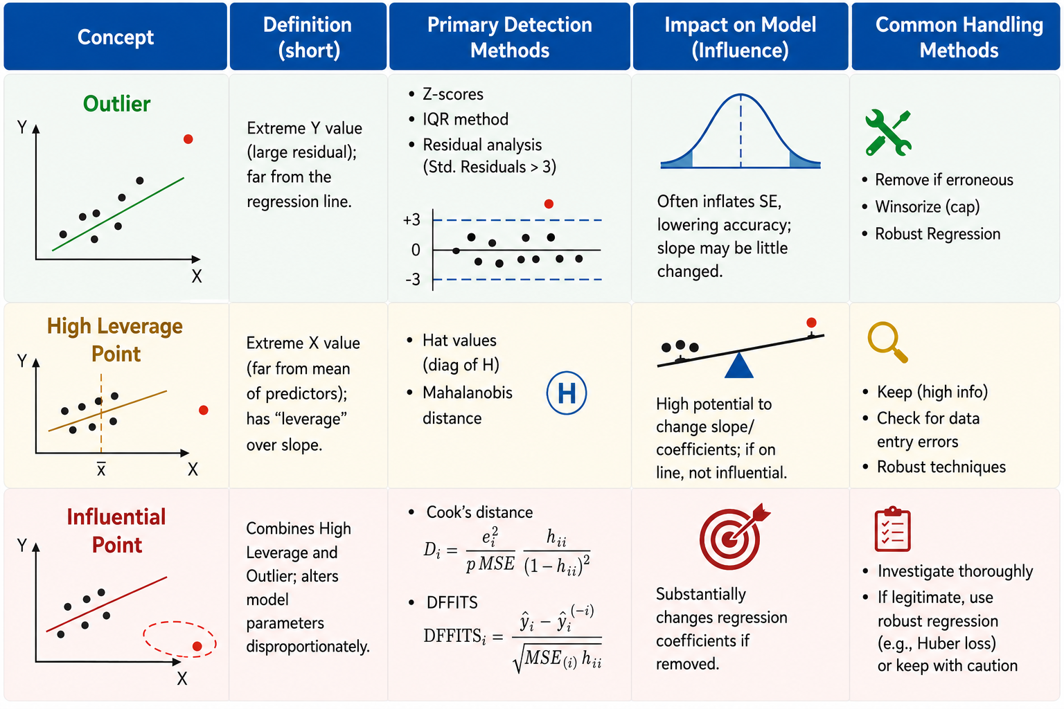
In Regression Analysis with labeled pairs: \(\{(\text{x}_i,y_i)\}_{i=1}^n\):
- Outliers are pairs \((\text{x}_i,y_i)\) with extreme \(y_i\).
- High leverage points are \((\text{x}_i,y_i)\) with extreme \(\text{x}_i\).
- High influential points: are all points \((\text{x}_i,y_i)\) that alters the analysis (predictions, slop coefficients, test results…).

Read, for example, Penn State STAT 462 Course Notes

Outliers/High leverage/Influential points

Outliers, high leverage and high influential points.

Handling influential points

Not all outliers or high leverage points would affect the analysis but influential points do.
We can apply capping (limiting extreme values to some threshold) or Trimming (completely remove them).
Some transformations may help reducing their effects:
- Z-score: \(x\to \frac{x-\overline{x}}{\sigma_{x}}\) (centered by mean, scaled by std).
- Min-Max scaling: \(x\to\frac{x-\min}{\max-\min}\in [0,1]\).
- If the data are positive: \(x\to \log(x)\) or \(x\to \sqrt{x}\)
No absolute solution! It depends on the analysis.

One-hot encoding

Consider gapminder dataset (2007).

Code

from gapminder import gapminder
import numpy as np
from sklearn.preprocessing import OneHotEncoder as onehot
encoder = onehot()
encoded_data = encoder.fit_transform(gapminder.loc[gapminder.year == 2007, ['continent']]).toarray()

# encoded dataset
X_encoded = pd.DataFrame(encoded_data, columns=[x.replace('continent_', '') for x in encoder.get_feature_names_out(['continent'])])
df_encoded = X_encoded.copy()
df_encoded['lifeExp'] = gapminder.lifeExp.loc[gapminder.year==2007].values
sorted_order = gapminder[gapminder.year == 2007].groupby('continent')['lifeExp'].median().sort_values().index
fig_cont = px.box(data_frame=gapminder.loc[gapminder.year==2007,:],
                  x="continent", y="lifeExp", color="continent",
                  category_orders={'continent': sorted_order})
fig_cont.update_layout(
    {'paper_bgcolor': 'rgba(0, 0, 0, 0)',
    'plot_bgcolor': 'rgba(42, 77, 152, 0)'},
    title="Life Expectancy vs Continent", 
    height=350, width=370)
fig_cont.update_xaxes(
    showline=True, 
    linewidth=1, 
    linecolor='gray',
    mirror=True,  # Mirrors the bottom x-axis line to the top
    showgrid=True, gridwidth=1, gridcolor=LIGHT_GRAY
)
fig_cont.update_yaxes(
    showline=True, 
    linewidth=1, 
    linecolor='gray', 
    mirror=True,  # Mirrors the left y-axis line to the right
    showgrid=True, gridwidth=1, gridcolor=LIGHT_GRAY
)
fig_cont.show()

Sometimes, categorical data are very informative and useful especially for building predictive models.
One-hot encoding is a way to covert them into numbers, especially for parametric model (linear regression…).
Ex: [‘Asia’, ‘Europe’, ‘Africa’]:

	Africa	Asia	Europe
0	0.0	1.0	0.0
1	0.0	0.0	1.0
2	1.0	0.0	0.0

4 Real Example

4.1 Real Example

Titanic Dataset (891 rows, 12 columns)

Survived	Pclass	Sex	Age	SibSp	Parch	Fare	Cabin	Embarked
0	3	male	34.500000	0	0	7.829200	nan	Q

Data types:

Survived	Pclass	Sex	Age	SibSp	Parch	Fare	Cabin	Embarked
int64	int64	object	float64	int64	int64	float64	object	object

Missing values:

Survived	Pclass	Sex	Age	SibSp	Parch	Fare	Cabin	Embarked
0	0	0	86	0	0	1	327	0

Question: What should we do in the preprocessing step?
- Convert Survived and Pclass to be object.
- Missing values: drop 1 NA of Fare, remove column Cabin and study Age.

Titanic Dataset (891 rows, 12 columns)

Convert data types:

col_to_be_converted = ['Survived', 'Pclass']
for col in col_to_be_converted:
    data[col] = data[col].astype(object)
data[col_to_be_converted].dtypes.to_frame().T

	Survived	Pclass
0	object	object

Drop column Cabin:

data.drop(columns = ["Cabin"], inplace = True)

Drop 1 row with NA in Fare:

data.dropna(subset = ['Fare'], inplace = True)

Handle issues: smaller \(\rightarrow\) bigger.

Study missing values in Age:
- Impact on qual. columns:

Code

import plotly.graph_objects as go
from plotly.subplots import make_subplots
import pandas as pd
import seaborn as sns
import matplotlib.pyplot as plt
sns.set(style="whitegrid")


# Assuming your DataFrame is named 'data'
data_dropna = data.dropna()
col_qual = ['Survived', 'Pclass', 'Sex', 'Embarked']

# 1. Initialize the 2x4 subplot grid
fig = make_subplots(rows=2, cols=4, 
                    vertical_spacing=0.2, 
                    horizontal_spacing=0.08)

for i, va in enumerate(col_qual):
    # --- Row 1: Before NA Removal ---
    # Calculate proportions (equivalent to stat="proportion")
    prop_before = data[va].value_counts(normalize=True).sort_index()
    
    fig.add_trace(
        go.Bar(
            x=prop_before.index.astype(str),
            y=prop_before.values,
            text=prop_before.values,
            texttemplate='%{text:.2f}', # Format to 2 decimal places
            textposition='outside',
            marker_color='#4C72B0',     # Matches Seaborn's default blue
            showlegend=False
        ),
        row=1, col=i+1
    )
    # Set X-axis title for the top row
    fig.update_xaxes(title_text=va, row=1, col=i+1)

    # --- Row 2: After NA Removal ---
    # Calculate proportions
    prop_after = data_dropna[va].value_counts(normalize=True).sort_index()
    
    fig.add_trace(
        go.Bar(
            x=prop_after.index.astype(str),
            y=prop_after.values,
            text=prop_after.values,
            texttemplate='%{text:.2f}', 
            textposition='outside',
            marker_color='#4C72B0',
            showlegend=False
        ),
        row=2, col=i+1)
    # Set X-axis title for the bottom row
    fig.update_xaxes(title_text=va, row=2, col=i+1)

# 2. Add Y-axis labels only to the first column (mimicking your if-statement)
fig.update_yaxes(title_text="Before remove NA", row=1, col=1)
fig.update_yaxes(title_text="After remove NA", row=2, col=1)

# 3. Uniformly scale Y-axes to ensure 'outside' text doesn't get clipped
fig.update_yaxes(range=[0, 1.15])

# 4. Polish the layout to mimic sns.set(style="whitegrid")
fig.update_layout(
    {'paper_bgcolor': 'rgba(0, 0, 0, 0)',
    'plot_bgcolor': 'rgba(42, 77, 152, 0)'},
    height=350,  # Adjust overall figure height
    width=420,   # Adjust overall figure width
    margin=dict(t=30, l=60, r=20, b=40)
)
fig.show()

Titanic Dataset (891 rows, 12 columns)

Impact on quan. columns:

Code

import plotly.graph_objects as go
from plotly.subplots import make_subplots
import numpy as np

# Assuming your DataFrame is named 'data'
data_dropna = data.dropna()
col_quan = ['SibSp', 'Parch', 'Fare']

# 1. Initialize the 2x3 subplot grid
fig_quan = make_subplots(rows=2, cols=3, 
                    vertical_spacing=0.22, 
                    horizontal_spacing=0.08)

for i, va in enumerate(col_quan):
    # Setup data targets for both rows
    datasets = [
        {"df": data[va].dropna(), "row": 1}, 
        {"df": data_dropna[va], "row": 2}
    ]
    
    # Identify the reference X-axis for this column (x, x2, x3)
    match_axis = 'x' if i == 0 else f'x{i+1}'
    
    for set_idx, target in enumerate(datasets):
        df_series = target["df"]
        curr_row = target["row"]
        curr_col = i + 1
        
        # Calculate Statistics
        mean_val = df_series.mean()
        median_val = df_series.median()
        std_val = df_series.std()
        
        # Add Histogram
        fig_quan.add_trace(
            go.Histogram(
                x=df_series, 
                histnorm='percent',
                marker_color='#4C72B0', 
                opacity=0.6, 
                showlegend=False
            ),
            row=curr_row, col=curr_col
        )
        
        show_in_legend = True if (curr_row == 1 and curr_col == 1) else False
        
        # Add Mean Vertical Line
        fig_quan.add_vline(
            x=mean_val, 
            line_width=2, 
            line_dash="dash", 
            line_color="#E66101", 
            name="Mean",
            showlegend=show_in_legend,
            row=curr_row, col=curr_col
        )
        
        # Add Median Vertical Line
        fig_quan.add_vline(
            x=median_val, 
            line_width=2, 
            line_color="#5E3C99", 
            name="Median",
            showlegend=show_in_legend,
            row=curr_row, col=curr_col
        )
        
        # Add Stats Box Annotation
        stats_text = f"Mean: {mean_val:.2f}<br>Med: {median_val:.2f}<br>Std: {std_val:.2f}"
        fig_quan.add_annotation(
            xref="x domain", yref="y domain",
            x=0.95, y=0.95,
            text=stats_text,
            showarrow=False,
            align="left",
            font=dict(size=10, color="black"),
            bordercolor="gray",
            borderwidth=1,
            borderpad=4,
            bgcolor="rgba(255, 255, 255, 0.8)", 
            row=curr_row, col=curr_col
        )
        
        # FIX: Added matches=match_axis to force identical x-ranges per column
        fig_quan.update_xaxes(title_text=va, matches=match_axis, row=curr_row, col=curr_col)

# 2. Add Y-axis labels only to the first column
fig_quan.update_yaxes(title_text="Percent (Before)", row=1, col=1)
fig_quan.update_yaxes(title_text="Percent (After)", row=2, col=1)

# 3. Polish the layout
fig_quan.update_layout(
    {'paper_bgcolor': 'rgba(0, 0, 0, 0)',
     'plot_bgcolor': 'rgba(42, 77, 152, 0)'},
    template="plotly_white",
    title="Quantitative Features Distribution Comparison",
    height=350, # Increased for readability
    width=450,  
    margin=dict(t=60, l=60, r=20, b=40),
    legend=dict(orientation="h", yanchor="bottom", y=1.02, xanchor="right", x=1)
)

fig_quan.show()

Study missing values in Age:
- Impact on qual. columns:

Code

fig.show()

Do you think that removing NA greatly affects other columns?

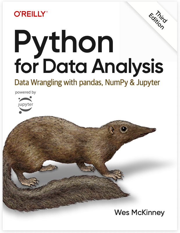
Read, for example, Chapter 7 of Python for Data Analysis by Wes McKinney.

Titanic Dataset (891 rows, 12 columns)

Dropping NA barely impacts other columns, it may be MCAR.

Simple Imputation

Median imputation (there are outliers).

data.fillna(value = data[['Age']].median(), inplace = True)
data.iloc[:,[1,2,4,5,6,7,9,10]].isna().sum().to_frame().T.style.hide()

Survived	Pclass	Sex	Age	SibSp	Parch	Fare	Embarked
0	0	0	0	0	0	0	0

Titanic Dataset (891 rows, 12 columns)

Dropping NA barely impacts other columns, it may be MCAR.

Model-based Imputation

Correlation analysis.

Code

data0['Family size'] = data0['SibSp'] + data0['Parch'] + 1
data0[['Age', 'Family size', 'Fare']].corr()\
    .style.background_gradient(cmap='coolwarm')

	Age	Family size	Fare
Age	1.000000	-0.090209	0.337932
Family size	-0.090209	1.000000	0.249924
Fare	0.337932	0.249924	1.000000

Pearson correlation.

Code

data0['Family size'] = data0['SibSp'] + data0['Parch'] + 1
data0[['Age', 'Family size', 'Fare']].corr('spearman')\
    .style.background_gradient(cmap='coolwarm')

	Age	Family size	Fare
Age	1.000000	-0.047033	0.315220
Family size	-0.047033	1.000000	0.503425
Fare	0.315220	0.503425	1.000000

Spearman correlation.

Age vs categorical variables.

🔑 Continuous features seem more related to Age (non-linearly related with Fare) than categorical ones.

Titanic Dataset (891 rows, 12 columns)

Dropping NA barely impacts other columns, it may be MCAR.

Model-based Imputation

Fare vs Age analysis:

Code

data0_log = data0[['Age', 'Fare', 'Family size']].copy()
data0_log['Fare'] = np.log1p(data0['Fare'])
data_temp = pd.concat([
    data0[['Age', 'Fare']],
    data0_log[['Age', 'Fare']]
], axis=0)

data_temp['Type'] = ['Orinal'] * data0.shape[0] + ['Log'] * data0.shape[0]


# Build the Figure with Graph Objects
fig_scatter = go.Figure()

# Trace 0: Original Data (Visible by default)
fig_scatter.add_trace(
    go.Scatter(
        x=data_temp[data_temp['Type'] == 'Orinal']['Fare'],
        y=data_temp[data_temp['Type'] == 'Orinal']['Age'],
        mode='markers',
        name='Original',
        marker=dict(color='#4C72B0'),
        visible=True
    )
)

# Trace 1: Log Data (Hidden by default)
fig_scatter.add_trace(
    go.Scatter(
        x=data_temp[data_temp['Type'] == 'Log']['Fare'],
        y=data_temp[data_temp['Type'] == 'Log']['Age'],
        mode='markers',
        name='Log-transformation',
        marker=dict(color='#4C72B0'),
        visible=False
    )
)

# Define the Slider Steps
# Using dot notation ("xaxis.title.text") keeps your frame/grid lines from being wiped out
steps = [
    dict(
        label="Original",
        method="update",
        args=[{"visible": [True, False]},       # Show original, hide log
              {"xaxis.title.text": "Fare"}]     # Update X axis label
    ),
    dict(
        label="Log-transformation",
        method="update",
        args=[{"visible": [False, True]},       # Hide original, show log
              {"xaxis.title.text": "Log(Fare + 1)"}]
    )
]
sliders = [dict(
    active=0,
    currentvalue={"prefix": "Data: "},
    pad={"t": 20},      # Push slider down slightly
    steps=steps
)]

# Custom Styling & Layout Configuration
fig_scatter.update_layout(
    {'paper_bgcolor': 'rgba(0,0,0,0)',
     'plot_bgcolor': 'rgba(0,0,0,0)'},
    title='Age vs Fare',
    width=450, 
    height=320, # Kept exactly as requested
    sliders=sliders,
    xaxis=dict(title="Fare"),
    yaxis=dict(title="Age")
)

# Apply your exact custom axes frames and grid styles
fig_scatter.update_xaxes(
    showline=True, linewidth=1, linecolor='gray', mirror=True,
    showgrid=True, gridwidth=1, gridcolor=LIGHT_GRAY
)
fig_scatter.update_yaxes(
    showline=True, linewidth=1, linecolor='gray', mirror=True,
    showgrid=True, gridwidth=1, gridcolor=LIGHT_GRAY
)
fig_scatter.show()

Scatter of Age vs Fare.

Age vs categorical variables.

🔑 Continuous features seem more related to Age (non-linearly related with Fare) than categorical ones.

Titanic Dataset (891 rows, 12 columns)

Dropping NA barely impacts other columns, it may be MCAR.

Model-based Imputation

Model: \({\color{blue}{\text{Age}\sim\text{Fam}+\text{log(Fare)}}}\).

IterativeImputer:

Code

from sklearn.experimental import enable_iterative_imputer
from sklearn.impute import IterativeImputer, KNNImputer
from sklearn.linear_model import LinearRegression
sub_data0 = data0_log[['Age', 'Family size', 'Fare']].query("Fare >= 1")
lr = LinearRegression()
imputer = IterativeImputer(
    estimator=lr,
    max_iter=10)
sub_data0[['Age', 'Family size', 'Fare']] = imputer.fit_transform(sub_data0)
sub_data0.isna().sum().to_frame().T.style.hide()

Age	Family size	Fare
0	0	0

KNNImputer:

Code

from sklearn.experimental import enable_iterative_imputer
from sklearn.impute import IterativeImputer, KNNImputer
sub_data1 = data0_log[['Age', 'Family size', 'Fare']].query("Fare >= 1")
imputer = KNNImputer(n_neighbors=2)
sub_data1[['Age', 'Family size', 'Fare']] = imputer.fit_transform(sub_data0)
sub_data1.isna().sum().to_frame().T.style.hide()

Age	Family size	Fare
0	0	0

Code

fig_boxes = make_subplots(rows=2, cols=2, 
                    vertical_spacing=0.18, 
                    horizontal_spacing=0.08)

# Box0
fig_boxes.add_trace(
    fig_box0.data[0],
    row=1, col=1
)
fig_boxes.update_xaxes(
    title_text='Age by dropping NA.', row=1, col=1)

# Box1
fig_boxes.add_trace(
    go.Histogram(
            x=sub_data0['Age'],
            opacity=0.7, 
            histnorm='percent',
            showlegend=False
        ),
        row=2, col=1
)
fig_boxes.update_xaxes(
    title_text='Age with SimpleImputer.', row=2, col=1)

# Box2
fig_boxes.add_trace(
    go.Histogram(
            x=sub_data1['Age'],
            opacity=0.7, 
            histnorm='percent',
            showlegend=False
        ),
        row=1, col=2
)
fig_boxes.update_xaxes(
    title_text='Age with IterativeImputer.', row=1, col=2)

# Box2
fig_boxes.add_trace(
    go.Histogram(
            x=sub_data1['Age'],
            opacity=0.7, 
            histnorm='percent',
            showlegend=False
        ),
        row=2, col=2
)
fig_boxes.update_xaxes(
    title_text='Age with KNNImputer.', row=2, col=2)

fig_boxes.update_layout(
    title='Imputer Comparison',
    template='plotly_white',
    height=400,
    width=450,
    margin=dict(t=30, l=60, r=20, b=40)
)
fig_boxes.show()

Titanic Dataset (891 rows, 12 columns)

Dropping NA barely impacts other columns, it may be MCAR.

Model-based Imputation

Model: \({\color{blue}{\text{Age}\sim\text{Fam}+\text{log(Fare)}}}\).

IterativeImputer:

Code

from sklearn.experimental import enable_iterative_imputer
from sklearn.impute import IterativeImputer, KNNImputer
from sklearn.linear_model import LinearRegression
sub_data0 = data0_log[['Age', 'Family size', 'Fare']].query("Fare >= 1")
lr = LinearRegression()
imputer = IterativeImputer(
    estimator=lr,
    max_iter=10)
sub_data0[['Age', 'Family size', 'Fare']] = imputer.fit_transform(sub_data0)
sub_data0.isna().sum().to_frame().T.style.hide()

Age	Family size	Fare
0	0	0

KNNImputer:

Code

from sklearn.experimental import enable_iterative_imputer
from sklearn.impute import IterativeImputer, KNNImputer
sub_data1 = data0_log[['Age', 'Family size', 'Fare']].query("Fare >= 1")
imputer = KNNImputer(n_neighbors=2)
sub_data1[['Age', 'Family size', 'Fare']] = imputer.fit_transform(sub_data0)
sub_data1.isna().sum().to_frame().T.style.hide()

Age	Family size	Fare
0	0	0

Code

fig_boxes = make_subplots(rows=2, cols=2, 
                    vertical_spacing=0.18, 
                    horizontal_spacing=0.08)

fig_box00 = px.histogram(
    data,
    x='Age',
    nbins=20,
    histnorm='percent'
)
fig_box00.update_layout({
    'paper_bgcolor': 'rgba(0,0,0,0)',
    'plot_bgcolor': 'rgba(0,0,0,0)'},
    title = 'Age distribution after imputation',
    width=400, height=220)
# 2. Add the royal blue frame by mirroring the x and y axes
fig_box00.update_xaxes(
    showline=True, 
    linewidth=1, 
    linecolor='gray', 
    mirror=True,  # Mirrors the bottom x-axis line to the top
    showgrid=True, gridwidth=1, gridcolor=LIGHT_GRAY
)
fig_box00.update_yaxes(
    showline=True, 
    linewidth=1, 
    linecolor='gray', 
    mirror=True,  # Mirrors the left y-axis line to the right
    showgrid=True, gridwidth=1, gridcolor=LIGHT_GRAY
)

# Box0
fig_boxes.add_trace(
    fig_box00.data[0],
    row=1, col=1
)
fig_boxes.update_xaxes(
    title_text='Age by dropping NA.', row=1, col=1)

# Box1
fig_boxes.add_trace(
    go.Histogram(
            x=sub_data0['Age'],
            opacity=0.7, 
            nbinsx=30,
            histnorm='percent',
            showlegend=False
        ),
        row=2, col=1
)
fig_boxes.update_xaxes(
    title_text='Age with SimpleImputer.', row=2, col=1)

# Box2
fig_boxes.add_trace(
    go.Histogram(
            x=sub_data1['Age'],
            opacity=0.7, 
            nbinsx=30,
            histnorm='percent',
            showlegend=False
        ),
        row=1, col=2
)
fig_boxes.update_xaxes(
    title_text='Age with IterativeImputer.', row=1, col=2)

# Box3
fig_boxes.add_trace(
    go.Histogram(
            x=sub_data1['Age'],
            opacity=0.7, 
            nbinsx=30,
            histnorm='percent',
            showlegend=False
        ),
        row=2, col=2
)
fig_boxes.update_xaxes(
    title_text='Age with KNNImputer.', row=2, col=2)

fig_boxes.update_layout(
    title='Imputer Comparison',
    template='plotly_white',
    height=400,
    width=450,
    margin=dict(t=30, l=60, r=20, b=40)
)
fig_boxes.show()

III. Data Quality & Preprocessing

Resources

1 Data Sources

1.1 Data sources

Primary

Secondary

Format

Structured

Unstructured

2 Data Quality

2.1 Data quality

3 Data Preprocessing

3.1 Data preprocessing

Drop rows vs drop columns

3.2 Missing values

An example

Missing values (1)

Missing Completely At Random (MCAR)

Missing values (2)

Missing At Random (MAR)

Missing values (3)

Missing Not At Random (MNAR)

Handling missing values

Rules of Thumb

3.3 Outliers vs Leverage Points

Univerate outliers

Bivariate outliers & high leverage points

Outliers/High leverage/Influential points

Handling influential points

One-hot encoding

4 Real Example

4.1 Real Example

Titanic Dataset (891 rows, 12 columns)

Data types:

Missing values:

Titanic Dataset (891 rows, 12 columns)

Titanic Dataset (891 rows, 12 columns)

Titanic Dataset (891 rows, 12 columns)

Simple Imputation

Titanic Dataset (891 rows, 12 columns)

Model-based Imputation

Titanic Dataset (891 rows, 12 columns)

Model-based Imputation

Titanic Dataset (891 rows, 12 columns)

Model-based Imputation

Titanic Dataset (891 rows, 12 columns)

Model-based Imputation

🥳 Yeahhhh….

Let’s Party… 🥂