import pandas as pd # Import pandas packageimport seaborn as sns # Package for beautiful graphsimport matplotlib.pyplot as plt # Graph managementdata = pd.read_csv(path_titanic +"/Titanic-Dataset.csv" ) # Import it into Pythonsns.set(style="whitegrid") # Set grid backgrounddata.drop(columns=['PassengerId']).head()
Survived
Pclass
Name
Sex
Age
SibSp
Parch
Ticket
Fare
Cabin
Embarked
0
0
3
Braund, Mr. Owen Harris
male
22.0
1
0
A/5 21171
7.2500
NaN
S
1
1
1
Cumings, Mrs. John Bradley (Florence Briggs Th...
female
38.0
1
0
PC 17599
71.2833
C85
C
2
1
3
Heikkinen, Miss. Laina
female
26.0
0
0
STON/O2. 3101282
7.9250
NaN
S
3
1
1
Futrelle, Mrs. Jacques Heath (Lily May Peel)
female
35.0
1
0
113803
53.1000
C123
S
4
0
3
Allen, Mr. William Henry
male
35.0
0
0
373450
8.0500
NaN
S
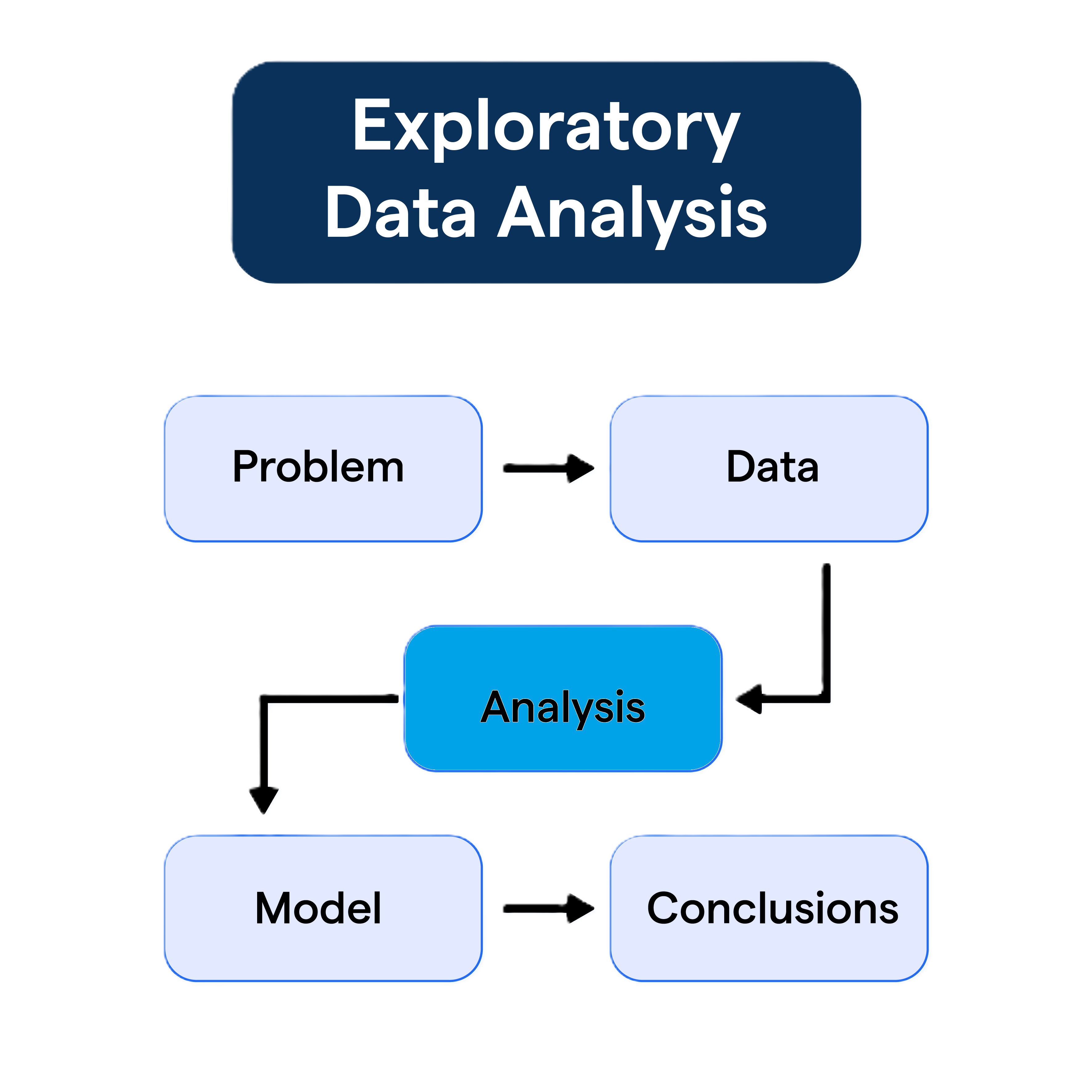
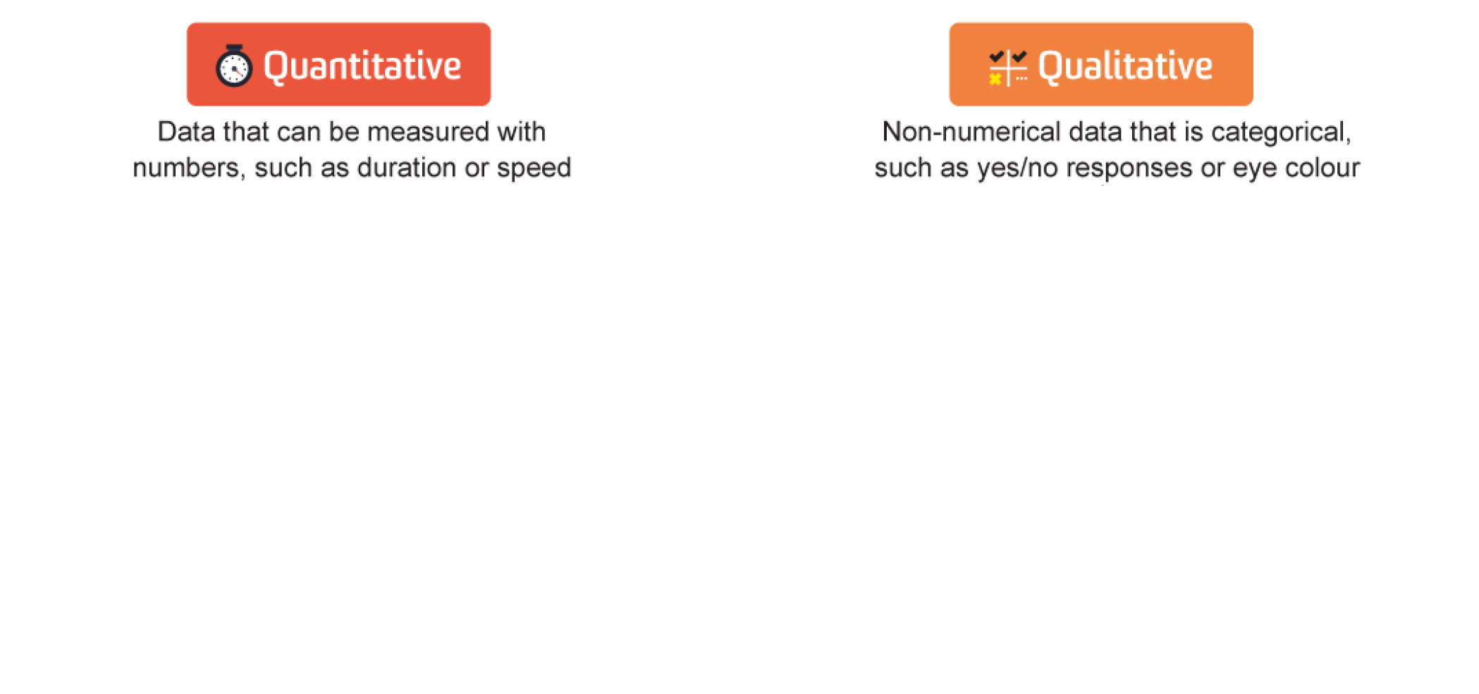
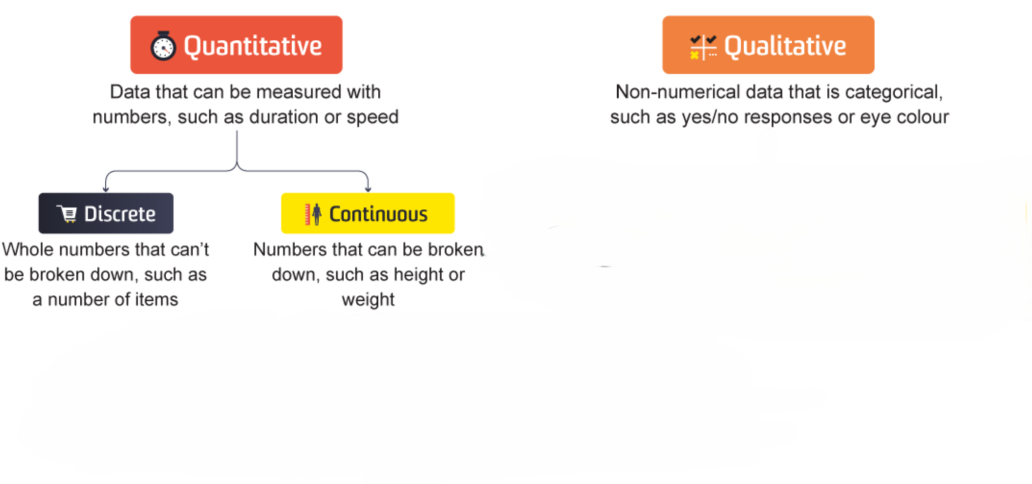
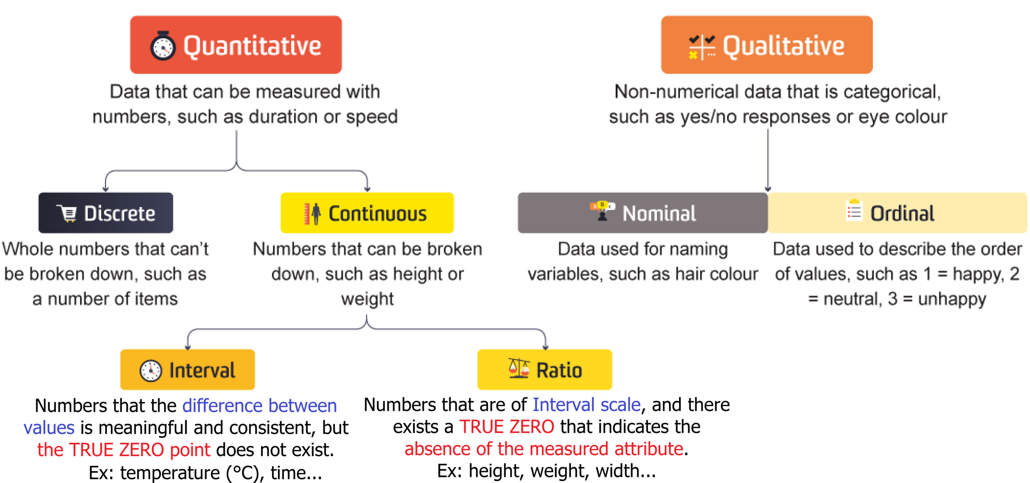
First step in analyzing data is understanding the nature of each individual column.
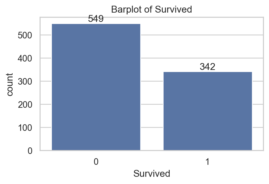
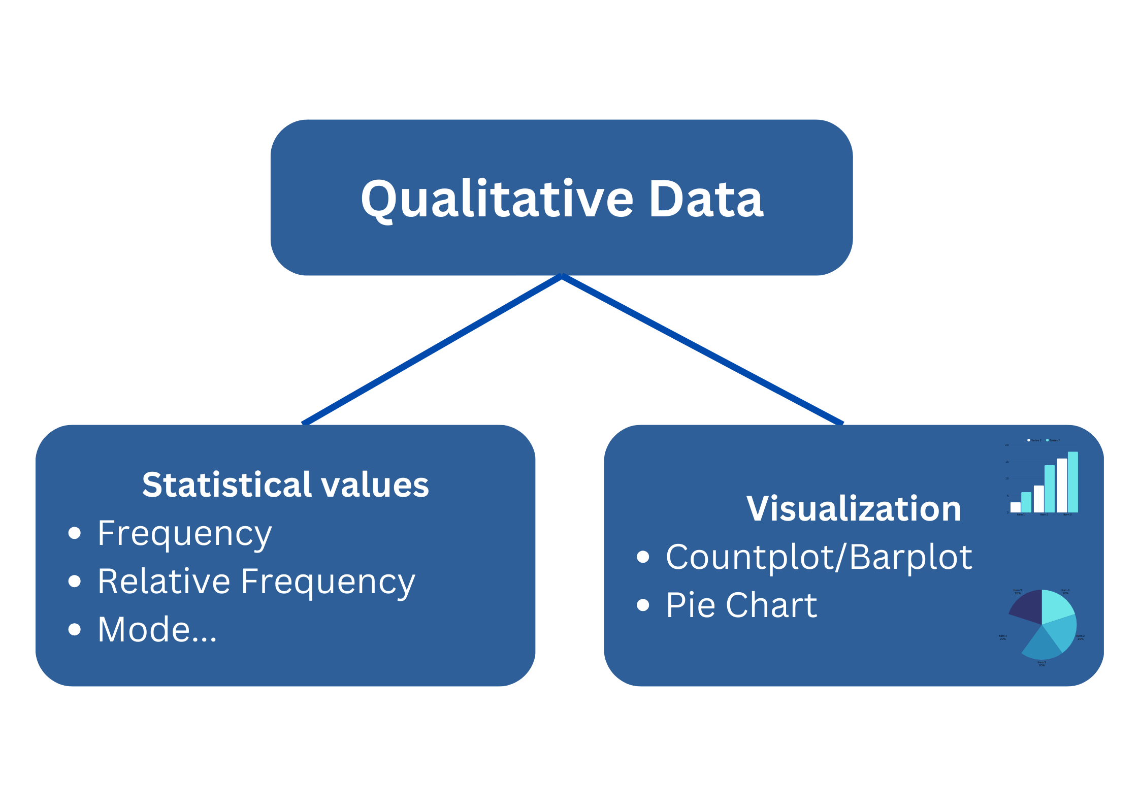
What graph should we use to present qualitative data?
Countplot/Barplot: Represent each count/proportion by a bar.
Example:
import matplotlib.pyplot as pltimport seaborn as sns # For graphsns.set(style="whitegrid") # set nice backgroundplt.figure(figsize=(5,3))ax = sns.countplot(data, x="Survived") # create graphax.set_title("Barplot of Survived") # add titleax.bar_label(ax.containers[0]) # add number to barsplt.show() # Show graph
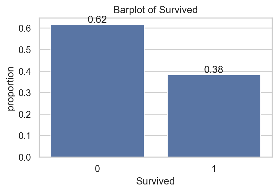
What graph should we use to present qualitative data?
Countplot/Barplot: Represent each count/proportion by a bar.
Example:
import matplotlib.pyplot as pltimport seaborn as sns # For graphsns.set(style="whitegrid") # set nice backgroundplt.figure(figsize=(5,3))ax = sns.countplot(data,x="Survived", stat="proportion")ax.set_title("Barplot of Survived") # add titleax.bar_label(ax.containers[0], fmt="%0.2f") # numberplt.show() # Show graph
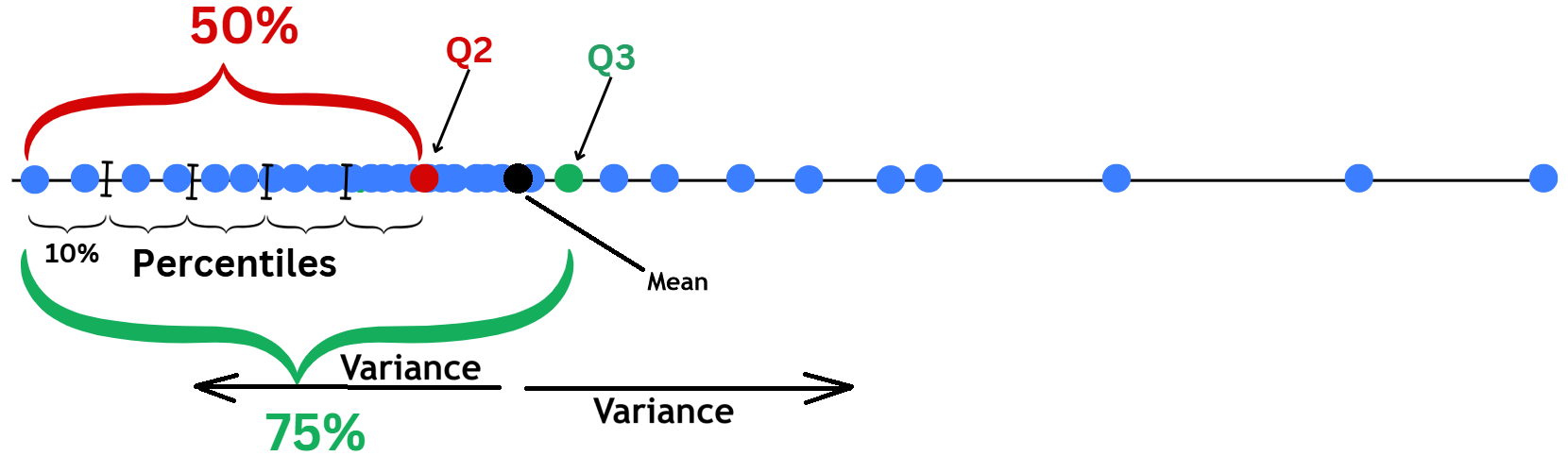
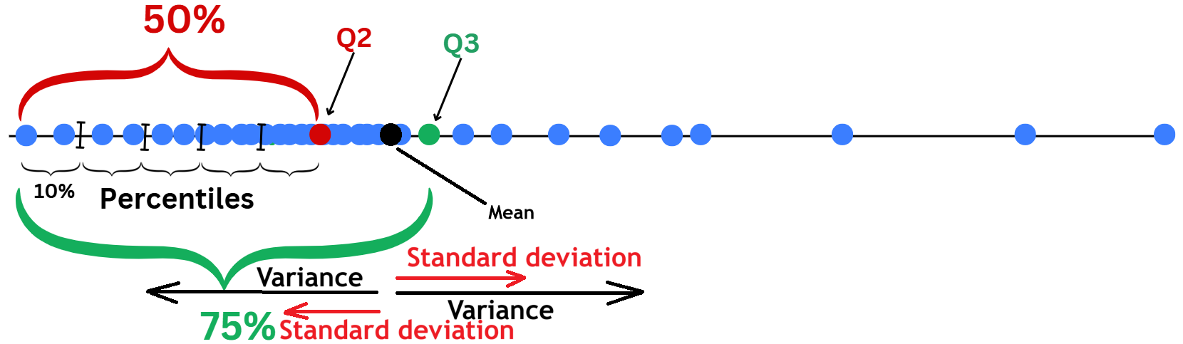
Large standard deviation (Std) means data points are spread out widely from the Mean.
Std has the same unit as \(X_i\).
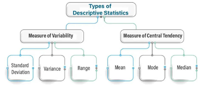
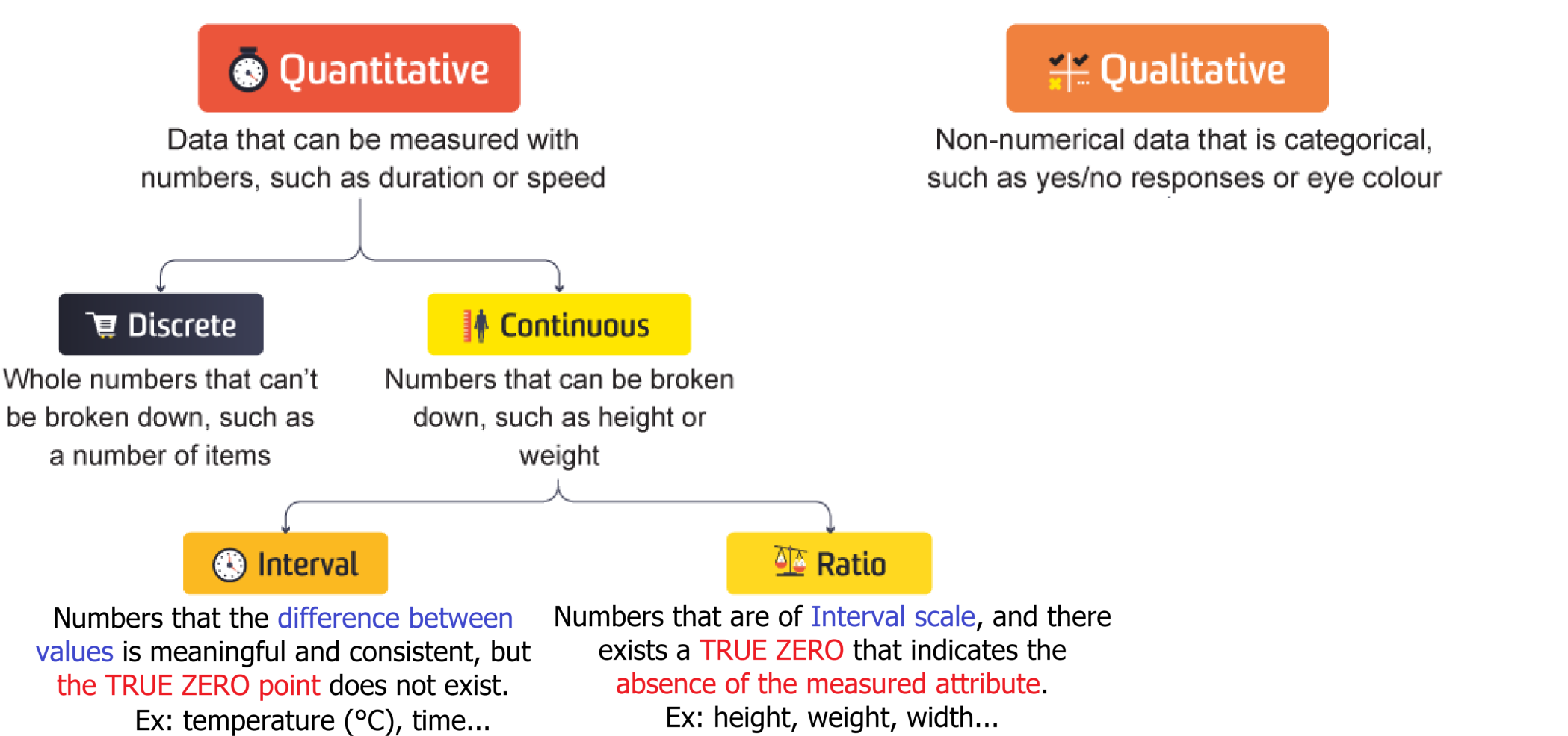
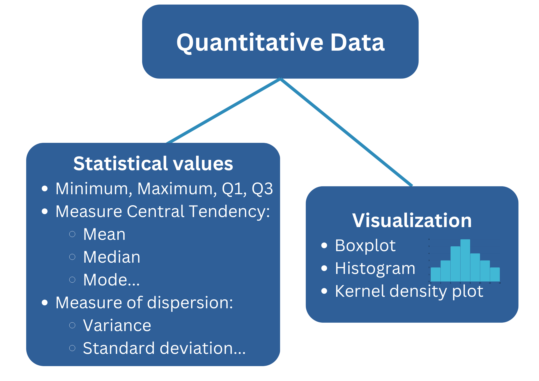
1.1.2. Quantitative Data
Statistical Summary
Age
Fare
SibSp
Parch
0
22.0
7.2500
1
0
1
38.0
71.2833
1
0
2
26.0
7.9250
0
0
3
35.0
53.1000
1
0
4
35.0
8.0500
0
0
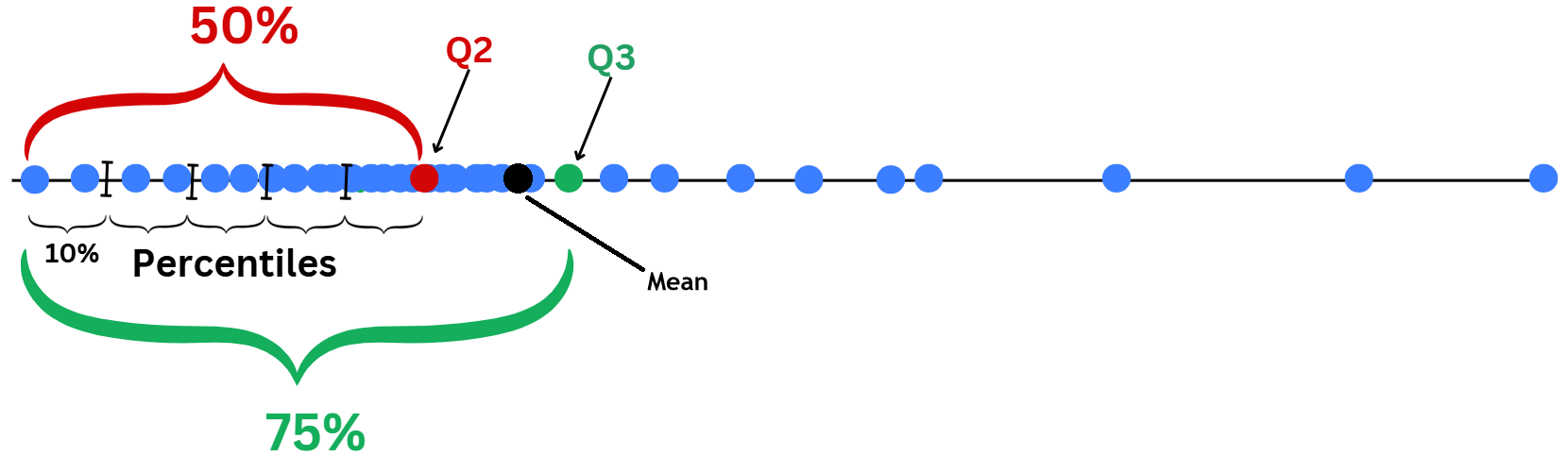
Statistical summary uses all key values to help us understand the data:
Where the data is concentrated (mean/median).
How spread out it is (var/std)…
Examples:
data[['Age','Fare']]\
        .describe().drop('count')  # for summary
Age
Fare
mean
29.699118
32.204208
std
14.526497
49.693429
min
0.420000
0.000000
25%
20.125000
7.910400
50%
28.000000
14.454200
75%
38.000000
31.000000
max
80.000000
512.329200
1.1.2. Quantitative Data
Visualization: Boxplot
Age
Fare
SibSp
Parch
0
22.0
7.2500
1
0
1
38.0
71.2833
1
0
2
26.0
7.9250
0
0
3
35.0
53.1000
1
0
4
35.0
8.0500
0
0
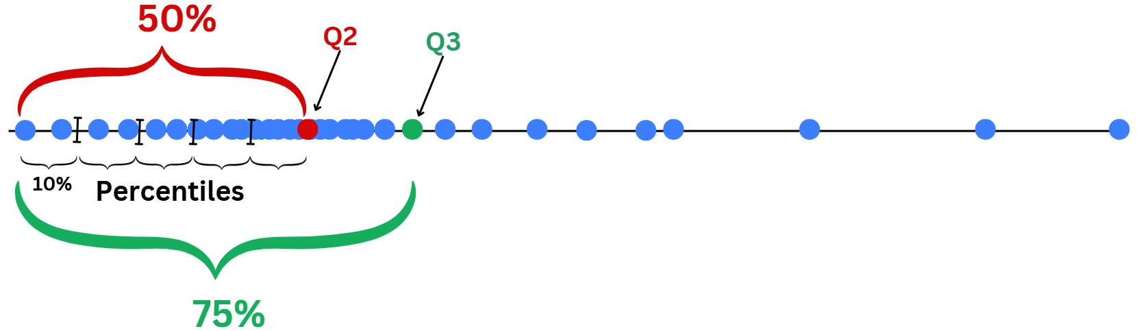
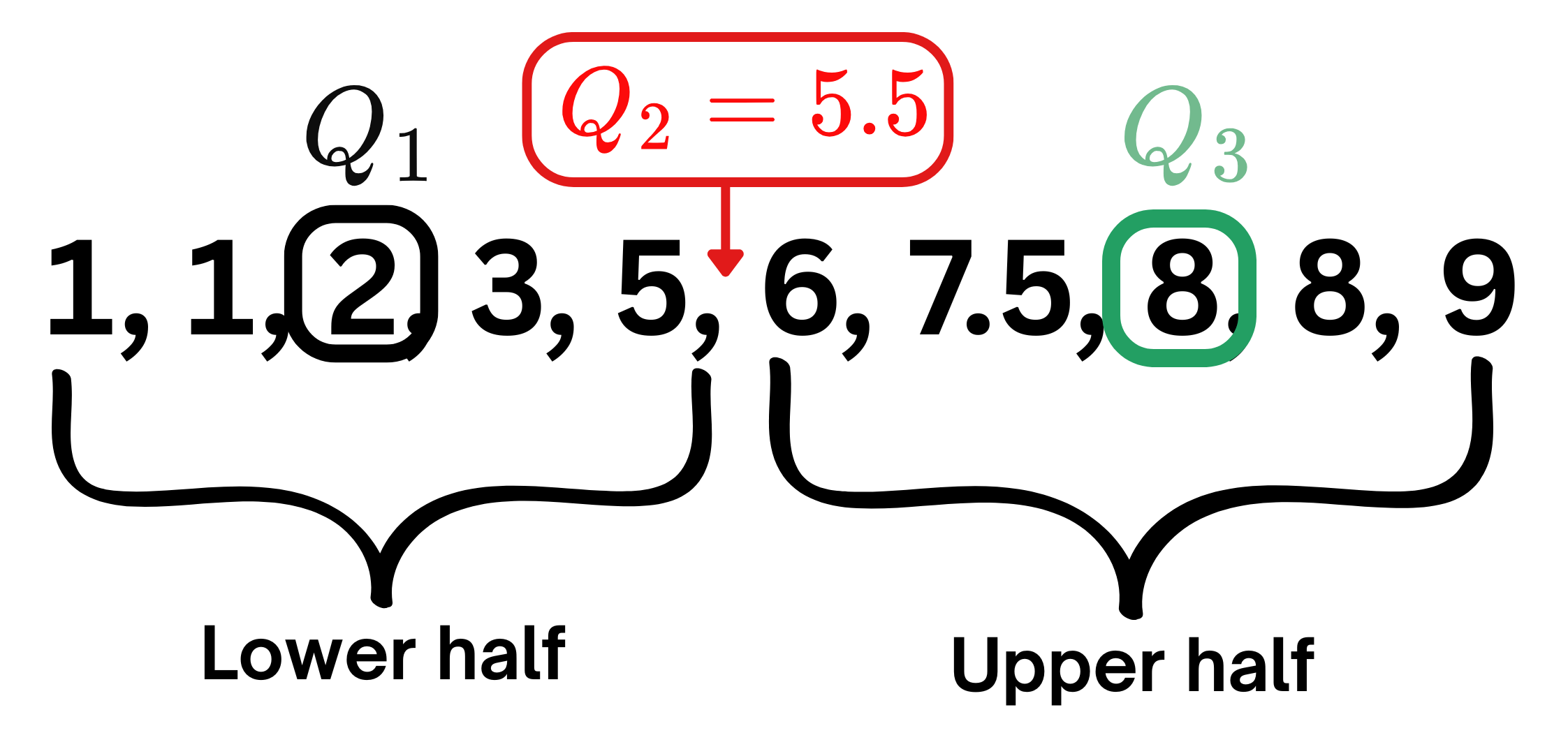
Boxplots describe data using Quartiles and the range where data normally fall within.
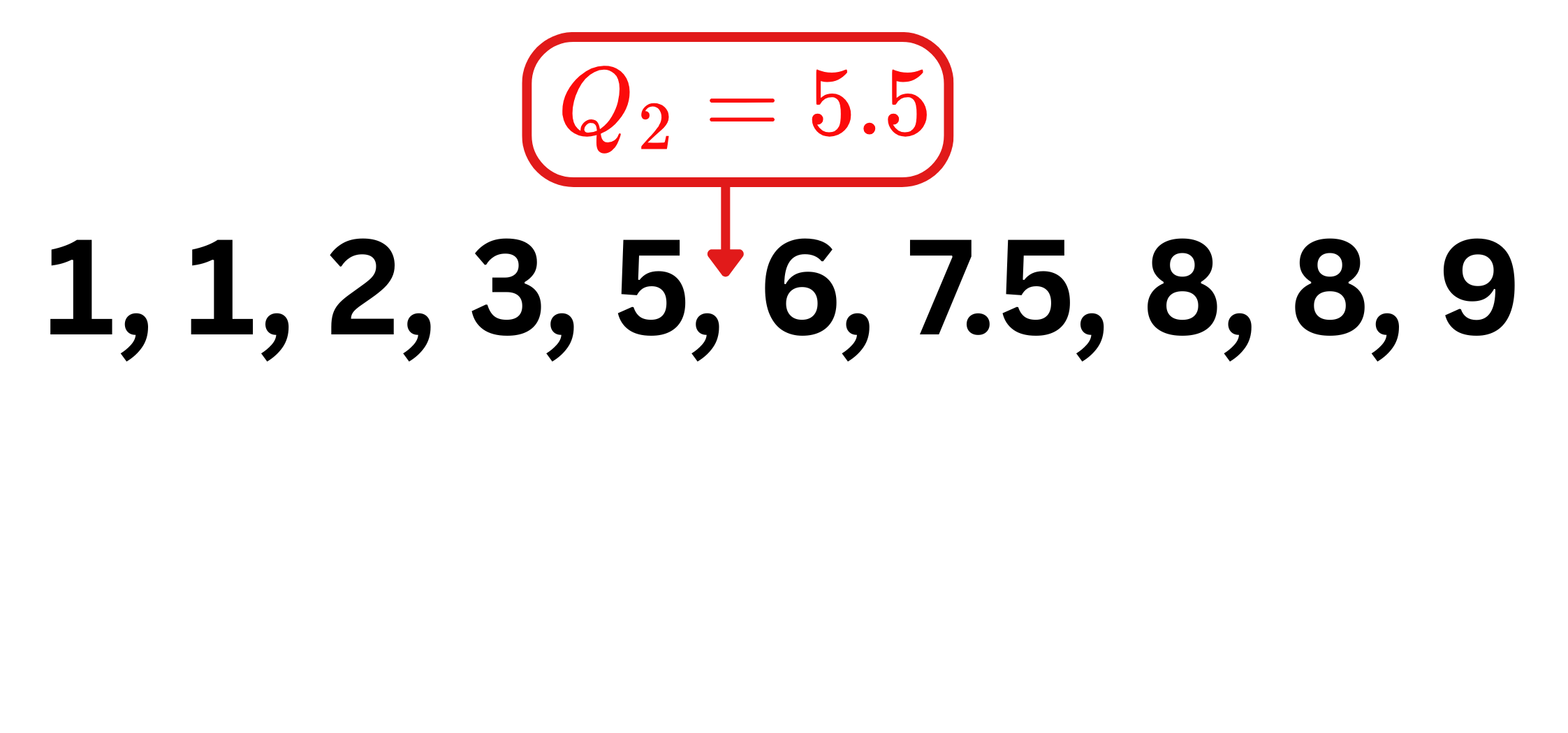
Lower and upper part of the box are \(Q_1\) and \(\color{green}{Q_3}\). Median\(\color{red}{Q_2}\) is the middle line.
Interquartile range:\(\text{IQR}=\color{green}{Q_3}-Q_1\), it’s the gap that covers central range of \(50\%\) of data.
Range:\([Q_1-1.5\text{IQR},\color{green}{Q_3}+1.5\text{IQR}]\). If the data is normally distributed, around 99.3% of the data would fall within this range.
Data points that fall outside this range, can be considered Outliers (data that deviate away from usual observations).
1.1.2. Quantitative Data
Visualization: Boxplot
Age
Fare
SibSp
Parch
0
22.0
7.2500
1
0
1
38.0
71.2833
1
0
2
26.0
7.9250
0
0
3
35.0
53.1000
1
0
4
35.0
8.0500
0
0
Code
import plotly.express as pxfig = px.box(data, x="Fare")fig.update_layout(height=220, width=530, title="Boxplot of Fare")fig.show()
Boxplots describe data using Quartiles and the range where data normally fall within.
Lower and upper part of the box are \(Q_1\) and \(\color{green}{Q_3}\). Median\(\color{red}{Q_2}\) is the middle line.
Interquartile range:\(\text{IQR}=\color{green}{Q_3}-Q_1\), it’s the gap that covers central range of \(50\%\) of data.
Range:\([Q_1-1.5\text{IQR},\color{green}{Q_3}+1.5\text{IQR}]\). If the data is normally distributed, around 99.3% of the data would fall within this range.
Data points that fall outside this range, can be considered Outliers (data that deviate away from usual observations).
1.1.2. Quantitative Data
Visualization: Boxplot
Code
import plotly.express as pxfig = px.box(data, x="Fare")fig.update_layout(height=220, width=530, title="Boxplot of Fare")fig.show()
This boxplot tells us that:
Fares range from \(£0\) to maximum fare of \(£512.33\).
\(Q_1=£7.9\) indicating that around \(25\%\) of passengers spent less than \(£7.9\) to get to the ship.
\(\color{red}{Q_2}=£14.45\) (Median): \(\approx 50\%\) spent less than \(£14.45\).
\(\color{green}{Q_3}=£31\): \(\approx 75\%\) spent less than \(£31\).
There are many outliers, passengers who spent more than the upper fence (\(£65\)), with the largest fare of \(£512.33\).
Boxplots describe data using Quartiles and the range where data normally fall within.
Lower and upper part of the box are \(Q_1\) and \(\color{green}{Q_3}\). Median\(\color{red}{Q_2}\) is the middle line.
Interquartile range:\(\text{IQR}=\color{green}{Q_3}-Q_1\), it’s the gap that covers central range of \(50\%\) of data.
Range:\([Q_1-1.5\text{IQR},\color{green}{Q_3}+1.5\text{IQR}]\). If the data are normally distributed, around 99.3% of the data would fall within this range.
Data points that fall outside this range, can be considered Outliers (data that deviate away from usual observations).
1.1.2. Quantitative Data
Visualization: Histogram
Code
import plotly.express as pxfig = px.histogram(data, x="Age")fig.update_layout(height=220, width=530, title="Histogram of Age")fig.show()
A histogram is constructed by:
Defining a grid range of bins: \(B_1, \dots, B_N\).
The height of each bar represents the count of \(X_i\) values that fall within the corresponding bin.
It describes the frequency of observations within each bin range.
Mathematical definition of histogram
Define bins: \(B_1,\dots, B_N\).
For any \(x\) and \(x\in B_k\) for some \(k\) then