KMeans & Hierarchical Clustering


CSCI-866-001: Data Mining & Knowledge Discovery


Lecturer: Dr. Sothea HAS

🗺️ Content

  • Introduction & Motivation

  • Kmeans as vector quantization

  • Hierarchical Clustering

  • Applications

Introduction & Motivation

Introduction & Motivation

Old Faithful dataset (\(272\) rows, \(2\) columns)

Code
import pandas as pd                 # Import pandas package
import seaborn as sns               # Package for beautiful graphs
import plotly.express as px
import matplotlib.pyplot as plt     # Graph management
# path = "https://gist.githubusercontent.com/curran/4b59d1046d9e66f2787780ad51a1cd87/raw/9ec906b78a98cf300947a37b56cfe70d01183200/data.tsv"                       # The data can be found in this link
df0 = pd.read_csv(path0 + "/faithful.csv" )  # Import it into Python
df0.head(5)                        # Randomly select 4 points
eruptions waiting
0 3.600 79
1 1.800 54
2 3.333 74
3 2.283 62
4 4.533 85

Code
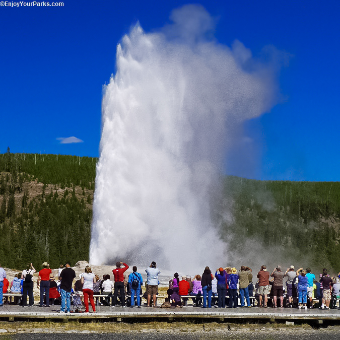
fig0 = px.scatter(df0, x="waiting", y="eruptions", size_max=50)    # Create scatterplot
fig0.update_layout(
    title="Old Faithful data from Yellowstone National Park, US",
    width=500, height=380)    # Title
fig0.show()
  • Two blocks: shorter wait & eruption, and the longer ones.

Introduction & Motivation

Satellite Image Segmentation

Introduction & Motivation

More motivations

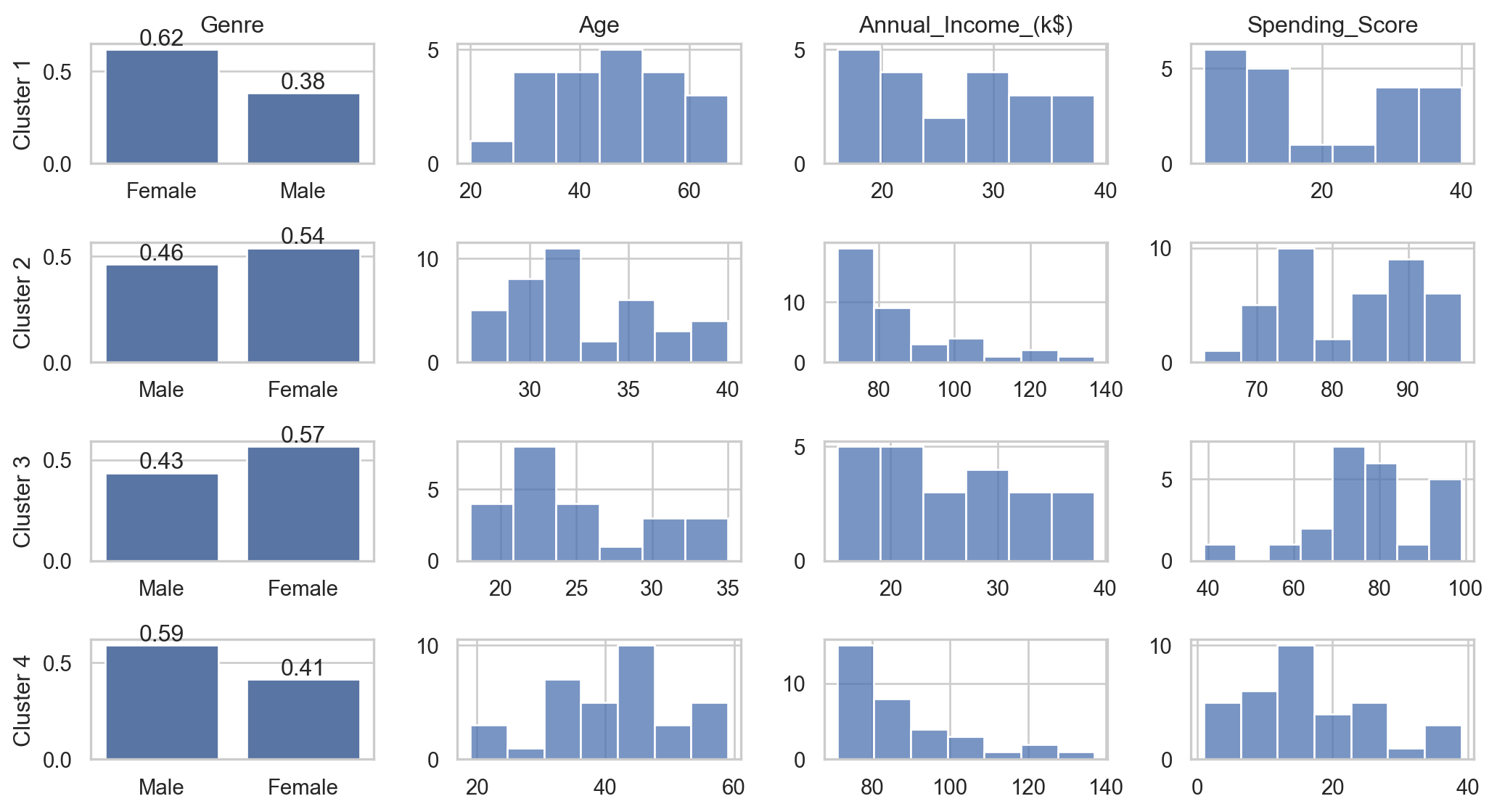
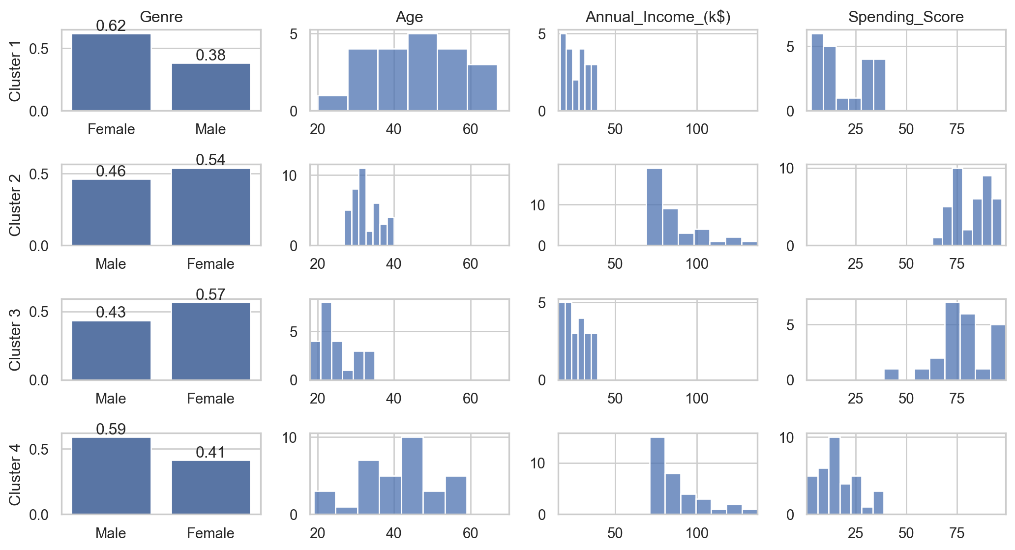
Marketing: finding groups of customers with similar behavior given a large database of customer data containing their properties and past buying records.

Biology: classification of plants and animals given their features.

Insurance: identifying groups of motor insurance policy holders with a high average claim cost; identifying frauds.

Bookshops: book ordering (recommendation).

City-planning: identifying groups of houses according to their type, value and geographical location.

Internet: document classification; clustering weblog data to discover groups of similar access patterns; topic modeling…

Introdution & Motivation

Clustering

Code
df0.head(2)
eruptions waiting
0 3.6 79
1 1.8 54
  • Clustering aims at partitioning a set of points from some metric space in such a way that

Introdution & Motivation

Clustering

Code
df0.head(2)
eruptions waiting
0 3.6 79
1 1.8 54
  • Clustering aims at partitioning a set of points from some metric space in such a way that
    • Points within the same group are close/similar, and

Introdution & Motivation

Clustering

Code
df0.head(2)
eruptions waiting
0 3.6 79
1 1.8 54
  • Clustering aims at partitioning a set of points from some metric space in such a way that
    • Points within the same group are close/similar, and
    • Points from different groups are distant.

Introdution & Motivation

Clustering

Code
df0.head(2)
eruptions waiting
0 3.6 79
1 1.8 54
  • Clustering aims at partitioning a set of points from some metric space in such a way that
    • Points within the same group are close/similar, and
    • Points from different groups are distant.
  • It belongs to the Unsupervised Learning branch of Machine Learning (ML).
  • Objective: group data into clusters based on their similarities.

Kmeans as a vector quantization

Kmeans as a vector quantization

Clustering as a compression problem

  • Given set of data \({\cal D}=\{\text{x}_1,\dots,\text{x}_n\}\subset\mathbb{R}^d\).
  • Compression: Represent \(\text{x}_i\) using a unique code-vector \(c_k\in{\cal C}=\{c_1,\dots,c_K\}\subset\mathbb{R}^d\) for some \(K\geq 1\).
eruptions waiting
0 3.600 79
1 1.800 54
2 3.333 74
3 2.283 62

Original data

eruptions waiting
0 4.298 80.285
1 2.094 54.750
2 4.298 80.285
3 2.094 54.750

Compressed data

  • Compression loss: \(\ell(\text{x}_i,c_k)=\|\text{x}_i-c_k\|^2=\sum_{j=1}^d(\text{x}_{ij}-c_{kj})^2.\)

Kmeans as a vector quantization

Problem setting

  • Compression loss: \(\ell(\text{x}_i,c_k)=\|\text{x}_i-c_k\|^2=\sum_{j=1}^d(\text{x}_{ij}-c_{kj})^2.\)
  • A \(K\)-point quantizer associated with codebook \(\cal C\) is any mapping:

\[\begin{align*}q:\mathbb{R}^d&\to{\cal C}=\{c_k:k=1,\dots,K\}\\ \text{x}_i&\mapsto q(\text{x}_i)=c_k\text{ for some }k.\end{align*}\]

  • We define Within Sum of Square criterion for a quantizer \(q\) by:

\[\color{red}{\text{WSS}}(q)=\sum_{i=1}^n\ell(\text{x}_i,q(\text{x}_i))=\sum_{i=1}^n\|\text{x}_i,q(\text{x}_i)\|^2.\]

  • Objective: find \(\color{blue}{q^*}\) that provides the lowest WSS, i.e.,

\[\color{red}{\text{WSS}}(\color{blue}{q^*})=\min_{q\in{\cal Q}}\color{red}{\text{WSS}}(q).\]

Kmeans as a vector quantization

Visualizing WSS

\[\color{red}{\text{WSS}}(q)=\sum_{i=1}^n\ell(\text{x}_i,q(\text{x}_i))=\sum_{i=1}^n\|\text{x}_i,q(\text{x}_i)\|^2.\]

  • Objective: find \(\color{blue}{q^*}\) that provides the lowest WSS, i.e.,

\[\color{red}{\text{WSS}}(\color{blue}{q^*})=\min_{q\in{\cal Q}}\color{red}{\text{WSS}}(q).\]

  • Quantizer \(q\) maps \(\text{x}_i\) to some centroid \(c_k\).
  • For k=1,2,...,K:
    • Within group k: \(\color{red}{\sum_{\text{x}_i\in G_k}\|\text{x}_i-c_k\|^2}.\)
  • \(\color{red}{\text{WSS}}(q)=\sum_{k=1}^K\color{red}{\sum_{\text{x}_i\in G_k}\|\text{x}_i-c_k\|^2}.\)

Measures the proximity of points within each group.

Kmeans as a vector quantization

Basic Identity WSS & Voronoi partition

For any number of cluster \(K\), one has: \[\color{blue}{\text{TSS}}=\color{green}{\text{BSS}}+\color{red}{\text{WSS}},\] where

  • \(\color{blue}{\text{TSS}}=\sum_{i=1}^n(\text{x}_i-\overline{\text{x}})^2\) and
  • \(\color{green}{\text{BSS}}=\sum_{k=1}^Kn_k(\overline{\text{x}}_k-\overline{\text{x}})^2.\)


  • If codebook \(\cal C=\{c_1,\dots,c_K\}\) is known, Voronoi partition associated with \(\cal C\) is defined by \[\color{green}{S_k}=\{\text{x}_i:\|\text{x}_i-\color{green}{c_k}\|\leq \|\text{x}_i-c_j\|, \forall j\neq k\}.\]

Kmeans as a vector quantization

Nearest Neighbor Condition

  • If codebook \({\cal C}=\{c_1,\dots,c_K\}\) is known, Voronoi partition associated with \(\cal C\) is defined by \[\color{green}{S_k}=\{\text{x}_i:\|\text{x}_i-\color{green}{c_k}\|\leq \|\text{x}_i-c_j\|, \forall j\neq k\}.\]

  • Given centroids \({\cal C}=\{c_1,\dots,c_K\}\), we can define groups by simply computing Voronoi partition.

Lemma 1: Nearet Neighbor Condition [Linder, T. (2002)]

Given a codebook \({\cal C}\), let \(q\) be any quantizer and \(\color{blue}{\hat{q}}\) be the quantizer that assigns any observation \(\text{x}_i\) to its closest code-vector (centroid of its Voronoi partition), i.e., \[\color{blue}{\hat{q}}(\text{x}_i)=\arg\min_{c_k\in{\cal C}}\|\text{x}_i-c_k\|^2\]

Then, one has \[\color{red}{\text{WSS}}(\color{blue}{\hat{q}})\leq \color{red}{\text{WSS}}(q).\]

Kmeans as a vector quantization

Centroid Condition

  • If codebook \({\cal C}=\{c_1,\dots,c_K\}\) is known, Voronoi partition associated with \(\cal C\) is defined by \[\color{green}{S_k}=\{\text{x}_i:\|\text{x}_i-\color{green}{c_k}\|\leq \|\text{x}_i-c_j\|, \forall j\neq k\}.\]

  • Given centroids \({\cal C}=\{c_1,\dots,c_K\}\), we can define groups by simply computing Voronoi partition.

Lemma 1: Centroid Condition [Linder, T. (2002)]

Given a partition \({\cal S}=\{S_1,\dots,S_K\}\), let \(q\) be any quantizer and \(\color{blue}{\hat{q}}\) be the quantizer with Voronoi parition and codebook \(\hat{{\cal C}}=\{\hat{c}_k\}\) defined by \[\hat{c}_k=\frac{1}{|S_k|}\sum_{\text{x}_i\in S_k}\text{x}_i.\]

Then, one has \[\color{red}{\text{WSS}}(\color{blue}{\hat{q}})\leq \color{red}{\text{WSS}}(q).\]

Kmeans as a vector quantization

Summary of Lemma 1

  • Nearet Neighbor Condition: Given codebook \({\cal C}=\{c_k\}\), we know how to assign \(\text{x}_i\mapsto c_k\) optimally, therefore find the best Voronoi parition.

  • Centroid Condition: Given a partition \({\cal S}=\{S_k\}\), we know how to define an optimal codebook \({\cal C}=\{c_k\}\).

  • Q1: Based on these results, how would you design a clustering algorithm?
  • A1: Something like: \({\cal C}_1\overset{\color{green}{\text{NNC}}}{\to}{\cal S}_1\overset{\color{red}{\text{CC}}}{\to}{\cal C}_2\overset{\color{green}{\text{NNC}}}{\to}{\cal S}_2...\)
  • This leads to the well-known KMeans clustering algorithm.

Kmeans as a vector quantization

KMeans Algorithm

  • Given data \({\cal D}=\{\text{x}_1,\dots,\text{x}_n\}\subset\mathbb{R}^d\) and \(K\).
  • Initialization: \({\cal C}^{0}=\{c_1,\dots,c_K\}\) (randomly).
  • Cluster Assignment (NNC):

for i = 1,...,n:
…. for k = 1,...,K: \[\text{Assign }\text{x}_i\to \color{green}{S_k}\text{ if }\|\text{x}_i-\color{green}{c_k}\|\leq \|\text{x}_i-c_j\|,\forall j\neq k.\]

  • Centroid Recomputation (CC): From \({\cal S}=\{S_k\}\) recompute new centroids:

\[c_k=\frac{1}{|S_k|}\sum_{\text{x}_i\in S_k}\text{x}_i.\]

  • Alternatively repeat step 2. and 3. until converges.
Code
from sklearn.cluster import KMeans
km = KMeans(n_clusters=4, init='random', max_iter=7, n_init=1, random_state=12)
km = km.fit(df1)
fig_km = go.Figure(go.Scatter(x=df1[:,0], y=df1[:,1], name="Data", mode="markers", 
                   marker=dict(color=[col1[str(j+1)] for j in km.labels_], size=7)))
fig_km.add_trace(go.Scatter(x=km.cluster_centers_[:,0], y=km.cluster_centers_[:,1],
                name="Centroid", mode="markers", marker=dict(color='black', size=15, symbol='star')))
fig_km.update_layout(width=500, height=480, title="KMeans Algorithm in Action")
fig_km.show()

Kmeans as a vector quantization

KMeans Algorithm may get stuck

  • Given data \({\cal D}=\{\text{x}_1,\dots,\text{x}_n\}\subset\mathbb{R}^d\) and \(K\).
  • Initialization: \(\color{red}{{\cal C}^{0}=\{c_1,\dots,c_K\}}\) (randomly).
  • Cluster Assignment (NNC):

for i = 1,...,n:
…. for k = 1,...,K: \[\text{Assign }\text{x}_i\to \color{green}{S_k}\text{ if }\|\text{x}_i-\color{green}{c_k}\|\leq \|\text{x}_i-c_j\|,\forall j\neq k.\]

  • Centroid Recomputation (CC): From \({\cal S}=\{S_k\}\) recompute new centroids:

\[c_k=\frac{1}{|S_k|}\sum_{\text{x}_i\in S_k}\text{x}_i.\]

  • Alternatively repeat step 2. and 3. until converges.
Code
from sklearn.cluster import KMeans
km = KMeans(n_clusters=4, init='random', max_iter=7, n_init=1, random_state=11)
km = km.fit(df1)
fig_km = go.Figure(go.Scatter(x=df1[:,0], y=df1[:,1], name="Data", mode="markers", 
                   marker=dict(color=[col1[str(j+1)] for j in km.labels_], size=7)))
fig_km.add_trace(go.Scatter(x=km.cluster_centers_[:,0], y=km.cluster_centers_[:,1],
                name="Centroid", mode="markers", marker=dict(color='black', size=15, symbol='star')))
fig_km.update_layout(width=500, height=480, title="KMeans Algorithm in Action")
fig_km.show()

Kmeans as a vector quantization

KMeans Algorithm may get stuck

  • Given data \({\cal D}=\{\text{x}_1,\dots,\text{x}_n\}\subset\mathbb{R}^d\) and \(K\).
  • A solution from KMeans of sklearn.cluster module:
from sklearn.cluster import KMeans
km = KMeans(
    n_clusters=4, 
    n_init=5     # Perform KMeans 5 times
)
km = km.fit(df1) # The best one among the 5

🔑 Perform KMeans n_init times with different random initializations, the best one (lowest WSS) is taken as the final result.

Q2: How to find a suitable \(K\)?

Code
fig_km1.show()

Kmeans as a vector quantization

Elbow Method

  • 🔑 \(\color{red}{\text{WSS}}\) decreases as \(K\) increases:
    • \(K=1\Rightarrow \color{red}{\text{WSS}}=\color{blue}{\text{TSS}}\)
    • \(K=n\Rightarrow \color{red}{\text{WSS}}=0\).
    • At the suitable \(K\), \(\color{red}{\text{WSS}}\) drops slowly.
Code
wss = []
list_k = list(range(1,11))
for k in list_k:
    km = KMeans(n_clusters = k, n_init=2)
    km = km.fit(df1)
    wss.append(km.inertia_)

data_wss = pd.DataFrame({
    'K' : list_k,
    'WSS': wss
})
fig6 = px.line(data_wss, x="K", y="WSS", markers="WSS", title="WSS vs Number of cluster (K)")
fig6.add_trace(go.Scatter(x=[4,4], y=[0,wss[3]], line=dict(color="red", dash="dash"),name="Optimal K"))
fig6.update_layout(width=500, height=280)
fig6.show()
Code
frames = []
for k in list_k[1:-2]: 
    km = KMeans(n_clusters=k, max_iter=100, n_init=2)
    km = km.fit(df1)
    frames.append(go.Frame(
        data=[go.Scatter(x=df1[:,0], y=df1[:,1], mode='markers', 
              marker=dict(color=km.labels_, size=7), 
              name=f'K: {k}'),
              go.Scatter(
                x=km.cluster_centers_[:,0],
                y=km.cluster_centers_[:,1],
                name="Centroid", mode="markers", 
                marker=dict(color='black', size=10, symbol='star'))],
        name=f'{k}'))

km = KMeans(n_clusters=2, max_iter=100, n_init=2)
km = km.fit(df1)
# Plotting
fig_km2 = go.Figure(
        data=[go.Scatter(x=df1[:,0], y=df1[:,1], mode='markers', 
              marker=dict(color=km.labels_, size=7)),
              go.Scatter(
                x=km.cluster_centers_[:,0],
                y=km.cluster_centers_[:,1],
                name="Centroid", mode="markers", 
                marker=dict(color='black', size=15, symbol='star'))],
        layout=go.Layout(
            title="KMeans iteration",
            xaxis=dict(title="X1", range=[-15, 7]),
            yaxis=dict(title="X2", range=[-15, 17]),
            updatemenus=[{
                "buttons": [
                    {
                        "args": [None, {"frame": {"duration": 1000, "redraw": True}, "fromcurrent": True, "mode": "immediate"}],
                        "label": "Play",
                        "method": "animate"
                    },
                    {
                        "args": [[None], {"frame": {"duration": 0, "redraw": False}, "mode": "immediate"}],
                        "label": "Stop",
                        "method": "animate"
                    }
                ],
                "type": "buttons",
                "showactive": False,
                "x": 0,
                "y": 1.25,
                "pad": {"r": 10, "t": 50}
            }],
            sliders=[{
                "active": 0,
                "currentvalue": {"prefix": "K: "},
                "pad": {"t": 50},
                "steps": [{"label": f"{i}",
                        "method": "animate",
                        "args": [[f'{i}'], {"frame": {"duration": 1000, "redraw": True}, "mode": "immediate", 
                        "transition": {"duration": 10}}]}
                        for i in list_k[1:-2]]
            }]
        ),
    frames=frames)

# Update layout
fig_km2.update_layout(
    width=450, height=450, 
    title="KMeans Algorithm with different K")

fig_km2.show()

Kmeans as a vector quantization

Silhouette Coefficients

🔑 If \(\color{blue}{\text{x}_i}\) belongs to cluster \(k\)-th, we define

  • \(a(\color{blue}{i})=\frac{1}{|S_k|-1}\sum_{j\neq i}\|\text{x}_j-\color{blue}{\text{x}_i}\|^2\): the proximity between \(\color{blue}{\text{x}_i}\) and other members within the same cluster.
  • \(b(\color{blue}{i})=\min_{j\neq k}\frac{1}{|S_j|}\sum_{\text{x}\in S_j}\|\text{x}-\color{blue}{\text{x}_i}\|^2\): proximity between \(\color{blue}{\text{x}_i}\) and other members of the nearest cluster.
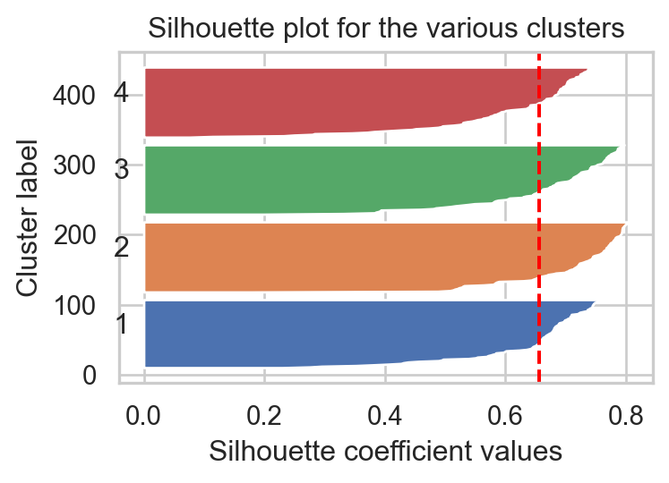
  • Silhouette value for any data point \(\color{blue}{\text{x}_i}\) is defined by: \[-1\leq s(\color{blue}{i})=\frac{b(\color{blue}{i})-a(\color{blue}{i})}{\max\{a(\color{blue}{i}),b(\color{blue}{i})\}}\leq 1.\]
    • \(s(\color{blue}{i})\approx 1\) indicates that the data point \(\color{blue}{\text{x}_i}\) is well-clustered within its cluster and distant from other groups.
    • \(s(\color{blue}{i})\approx -1\) indicates that the data point \(\color{blue}{\text{x}_i}\) is distant from other members of its cluster and should belong to the nearest group.
  • Silhouette Coefficient for a given \(K\) is \(\tilde{s}(K)=\sum_{i=1}^ns(i)/n.\)
  • Optimal number of cluster \(K^*=\arg\max_{K_\min\leq k\leq K_\max}\{\tilde{s}(k)\}.\)
Code
from sklearn.metrics import silhouette_score, silhouette_samples
km = KMeans(n_clusters=4, max_iter=100, n_init=2)
km = km.fit(df1)
clusters = km.labels_
silhouette_avg = silhouette_score(df1, clusters)
sample_silhouette_values = silhouette_samples(df1, clusters)

# Plot silhouette scores
fig, ax1 = plt.subplots(1, 1, figsize=(4,2.5))
y_lower = 10
for k in range(km.n_clusters):
    ith_cluster_silhouette_values = sample_silhouette_values[clusters == k]
    ith_cluster_silhouette_values.sort()
    size_cluster_k = ith_cluster_silhouette_values.shape[0]
    y_upper = y_lower + size_cluster_k
    ax1.fill_betweenx(np.arange(y_lower, y_upper), 0,
                      ith_cluster_silhouette_values)
    ax1.text(-0.05, y_lower + 0.5 * size_cluster_k, str(k+1))
    y_lower = y_upper + 10
ax1.set_title("Silhouette plot for the various clusters")
ax1.set_xlabel("Silhouette coefficient values")
ax1.set_ylabel("Cluster label")
ax1.axvline(x=silhouette_avg, color="red", linestyle="--")

Code
sc_av = []
for k in range(2,10):
  kmeans = KMeans(n_clusters=k, n_init=3)
  clusters = kmeans.fit_predict(df1)
  sc_av.append(silhouette_score(df1, clusters))
sc_df = pd.DataFrame({'k' : range(2, 10),
                      'Silhouette Coefficient' : sc_av})
fig6 = px.line(data_frame=sc_df, x='k', y='Silhouette Coefficient', markers='Silhouette Coefficient')
fig6.add_trace(go.Scatter(x=[4,4],y=[np.min(sc_av), np.max(sc_av)],  line=dict(dash="dash"), name=r"$K^*$"))
fig6.update_layout(width=300, height=180, title = "Silhouette Coefficient vs K")
fig6.show()

Kmeans as a vector quantization

Summary

  • KMeans involves two alternative processes:

    • Cluster assignment: \({\cal C}=\{c_k\}\to {\cal S}=\{S_k\}\).
    • Centroid recomputation: \({\cal S}=\{S_k\}\to{\cal C}=\{c_k\}\).
  • The algorithm may get stuck if it started from bad initialization. Increasing n_init may solves this problem.

  • A suitable number of cluster \(K\) may be estimated using:

    • Elbow method: Find the elbow of \(\color{red}{\text{WSS}}\) vs \(K\) curve.
    • Silhouette coefficient: find \(K\) that maximizes this coef.

Hierarchical clustering

Hierarchical clustering

Agglomerative clustering (Bottom-up)

  • It does not require the prior knowledge of \(K\).
  • Let \(\cal D=\{\text{x}_1,\dots, \text{x}_1\}\) be the data points.

Agglomerative clustering

  • Start: Each point belongs to its own cluster (\(K=n\)).
  • Merging: Pairs of clusters are merged as we move up.
  • End: All points are in one cluster.
  • At each step, \(\color{red}{\text{WSS}}\) is recorded.
  • As we move up, \(K\) decreases, the jump in \(\color{red}{\text{WSS}}\) should indicate the suitable number of cluster \(K\).
  • Q3: How to link clusters together?
  • A3: We need tools AKA “Linkages”.
Linkage Formula
Single Linkage \(d_{\text{SL}}(A, B) = \min \{ \|a, b\|^2 : a \in A, b \in B \}\)
Complete Linkage \(d_{\text{CoL}}(A, B) = \max \{ \|a, b\|^2 : a \in A, b \in B \}\)
Average Linkage \(d_{\text{AL}}(A, B) = \frac{1}{|A||B|} \sum_{a \in A} \sum_{b \in B} \|a, b\|^2\)
Centroid Linkage \(d_{\text{CeL}}(A, B) = \|\bar{a}, \bar{b}\|^2\) where \(\bar{a}\) and \(\bar{b}\) are centroids of clusters \(A\) and \(B\), respectively.
Ward’s Linkage \(d_{\text{WL}}(A, B) = \sqrt{\frac{|A||B|}{|A| + |B|} \| \bar{a} - \bar{b} \|^2}\)

Hierarchical clustering

Agglomerative clustering (Bottom-up)

Code
from scipy.cluster.hierarchy import dendrogram, linkage
from sklearn.cluster import AgglomerativeClustering
import seaborn as sns
fig, axs = plt.subplots(2,4, figsize=(14, 6))
data_linkage = linkage(df1, method='single')
dendrogram(data_linkage, ax=axs[0,0])
axs[0,0].set_title("Single Linkge")
axs[0,0].set_xticks([])
clust = AgglomerativeClustering(n_clusters=2).fit_predict(df1)
sns.scatterplot(x=df1[:,0], y=df1[:,1], c=[i+1 for i in clust], ax=axs[1,0])
axs[1,0].set_title("K = 2")

data_linkage = linkage(df1, method='complete')
dendrogram(data_linkage, ax=axs[0,1])
axs[0,1].set_title("Complete Linkge")
axs[0,1].set_xticks([])
clust = AgglomerativeClustering(n_clusters=3).fit_predict(df1)
sns.scatterplot(x=df1[:,0], y=df1[:,1], c=[i+1 for i in clust], ax=axs[1,1])
axs[1,1].set_title("K = 3")

data_linkage = linkage(df1, method='average')
dendrogram(data_linkage, ax=axs[0,2])
axs[0,2].set_title("Average Linkge")
axs[0,2].set_xticks([])
clust = AgglomerativeClustering(n_clusters=4).fit_predict(df1)
sns.scatterplot(x=df1[:,0], y=df1[:,1], c=[i+1 for i in clust], ax=axs[1,2])
axs[1,2].set_title("K = 4")

data_linkage = linkage(df1, method='ward')
dendrogram(data_linkage, ax=axs[0,3])
axs[0,3].set_title("Ward's Linkge")
axs[0,3].set_xticks([])
clust = AgglomerativeClustering(n_clusters=5).fit_predict(df1)
sns.scatterplot(x=df1[:,0], y=df1[:,1], c=[i+1 for i in clust], ax=axs[1,3])
axs[1,3].set_title("K = 5")
plt.show()

Applications

Applications

Image segmentation

  • Performance image segmentation on one channel of the follwoing image.
Code
from skimage import data
image = data.astronaut()
plt.imshow(image[:,:,1])
plt.axis('off')
plt.show()

Code
sns.set(style="white")
image_gray = image[:,:,1].reshape(-1,1)
_, ax = plt.subplots(2, 2, figsize=(7, 5.25))
for k in range(2, 6):
    km_image = KMeans(n_clusters=k)
    km_image_fit = km_image.fit(image_gray)
    image_compressed = np.array([np.mean(image_gray[km_image_fit.labels_==i]) for i in range(k)])
    image_seg = np.zeros_like(km_image_fit.labels_)
    for i in range(k):
        image_seg[km_image_fit.labels_ == i] = image_compressed[i]

    image_reshaped = image_seg.reshape(image.shape[0], image.shape[1])
    ax[(k-2)//2,(k-2)%2].imshow(image_reshaped, cmap='gray')
    ax[(k-2)//2,(k-2)%2].set_title(f"K = {k}")
    ax[(k-2)//2,(k-2)%2].axis('off')
plt.tight_layout()
plt.show()

Applications

Customer Segmentation: Credit Card dataset

Genre Age Annual_Income_(k$) Spending_Score
0 Male 19 15 39
1 Male 21 15 81
2 Female 20 16 6
3 Female 23 16 77
4 Female 31 17 40
  • Q4: What should you do in preprocessing step?

  • A4: Encode Genre, missing, duplicated values, scaling…

Applications

Customer Segmentation: Credit Card dataset

Missing values:
    Genre  Age  Annual_Income_(k$)  Spending_Score
0      0    0                   0               0

Applications

Can you interpret each group?

Applications

How about now?

Summary

  • Clustering is a key technique in the unsupervised learning branch of machine learning.

  • It plays a crucial role in tasks involving the organization and segmentation of data based on their similarities.

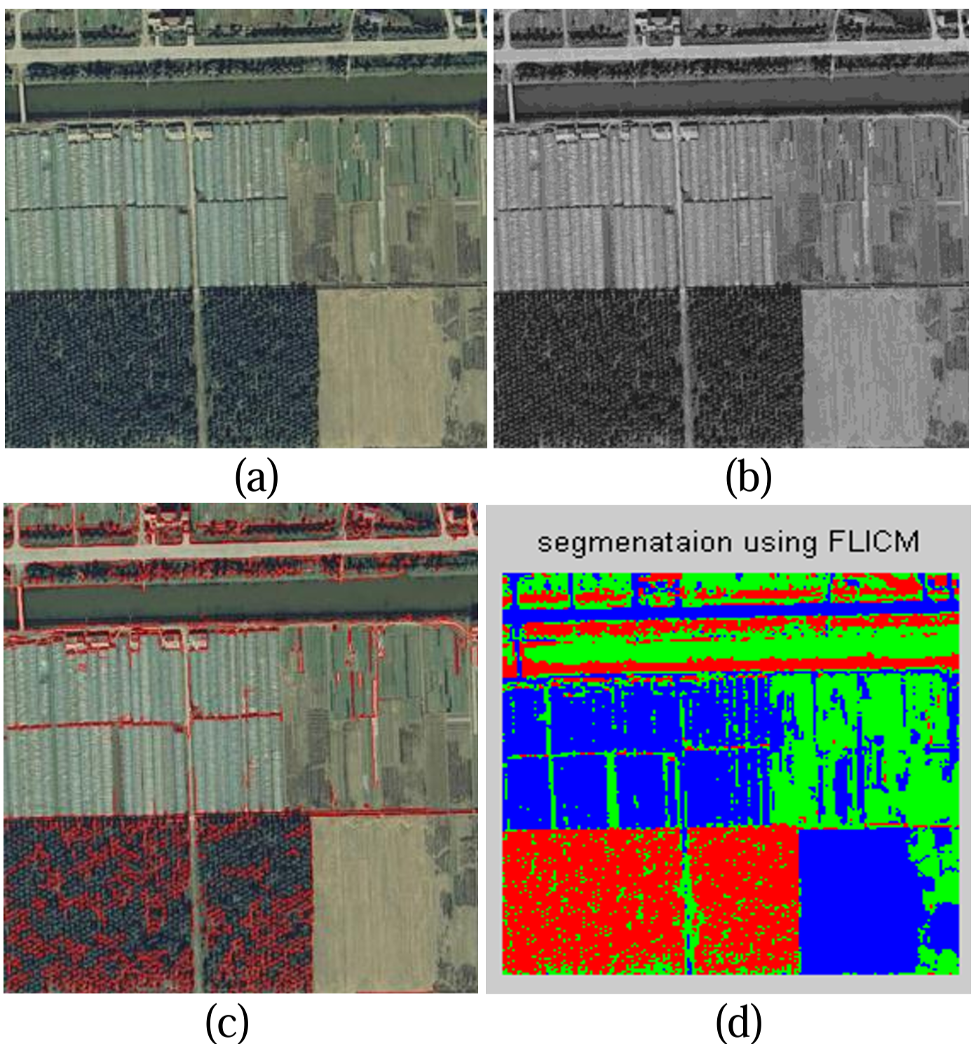
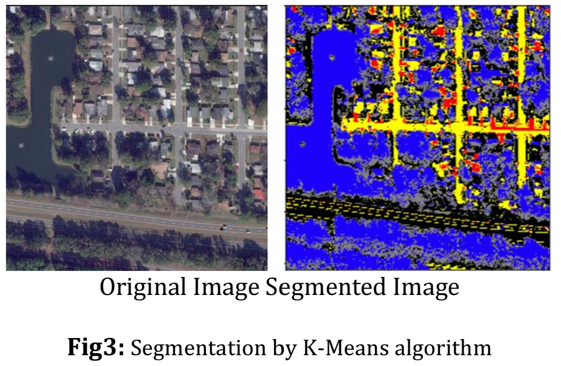
  • It can be applied in various fields such as market segmentation, image processing, and anomaly detection.

  • There are numerous clustering algorithms available, each suited to different types of data and purposes, such as KMeans, Hierarchical Clustering, DBSCAN, and Spectral Clustering.

  • Interpreting clustering results can be challenging, but it is an essential step to ensure the validity and usefulness of the clusters identified.

🥳 It’s party time 🥂