data = pd.read_csv(path + "/heart.csv")
quan_vars = ['age','trestbps','chol','thalach','oldpeak']
qual_vars = ['sex','cp','fbs','restecg','exang','slope','ca','thal','target']
# Convert to correct types
for i in quan_vars:
data[i] = data[i].astype('float')
for i in qual_vars:
data[i] = data[i].astype('category')
# Train test split
from sklearn.model_selection import train_test_split
data_no_dup = data.drop_duplicates()
X, y = data_no_dup.iloc[:,:-1], data_no_dup.iloc[:,-1]
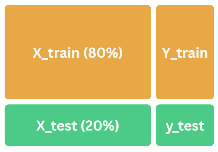
X_train, X_test, y_train, y_test = train_test_split(X, y, test_size=0.2, stratify=y, random_state=42)
from sklearn.model_selection import GridSearchCV
from sklearn.tree import DecisionTreeClassifier
from sklearn.metrics import accuracy_score
from sklearn.metrics import roc_auc_score, accuracy_score, precision_score, recall_score, f1_score, confusion_matrix, ConfusionMatrixDisplay
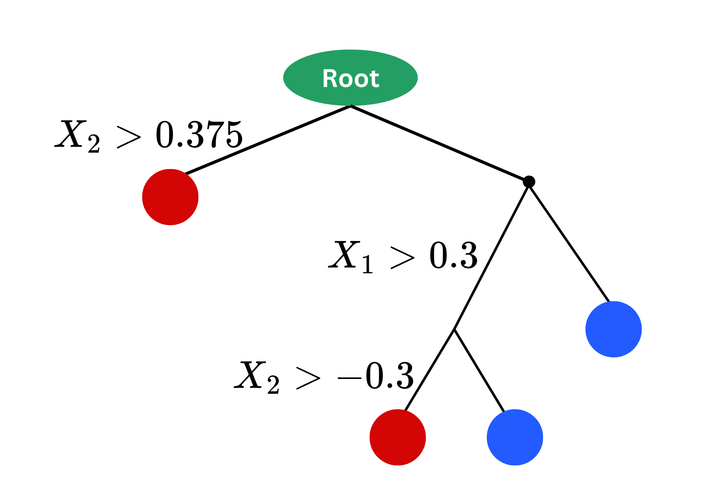
clf = DecisionTreeClassifier()
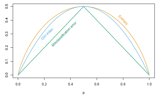
param_grid = {'criterion': ['gini', 'entropy'],
'min_samples_leaf': [2, 5, 10, 16, 20, 25, 30],
'max_features': ['auto', 'sqrt', 'log2', 2, 5, 10, X_train.shape[1]] }
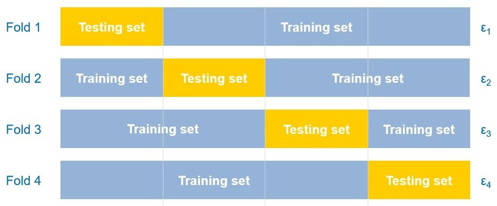
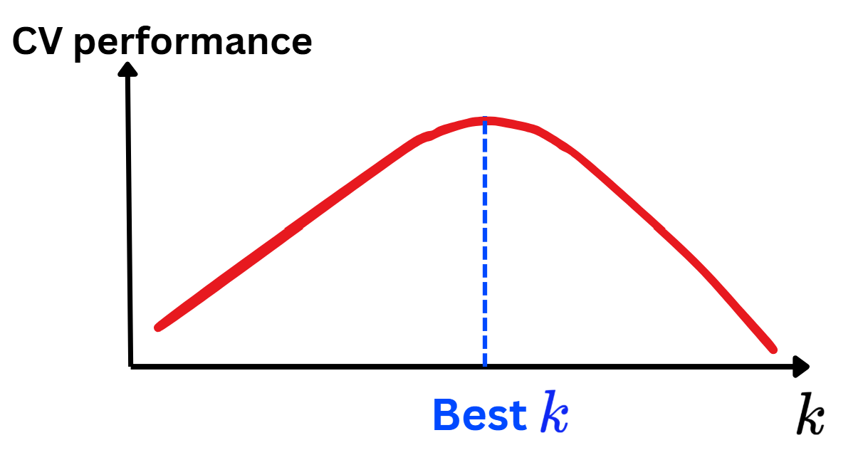
grid_search = GridSearchCV(estimator=clf, param_grid=param_grid, cv=10, scoring='accuracy', n_jobs=-1)
grid_search.fit(X_train, y_train)
best_model = grid_search.best_estimator_
y_pred = best_model.predict(X_test)
test_tr = pd.DataFrame(
data={'Accuracy': accuracy_score(y_test, y_pred),
'Precision': precision_score(y_test, y_pred),
'Recall': recall_score(y_test, y_pred),
'F1-score': f1_score(y_test, y_pred)},
columns=["Accuracy", "Precision", "Recall", "F1-score"],
index=["Tree"])
test_tr = pd.concat([test_tr, pd.DataFrame(
data={'Accuracy': 0.885246,
'Precision': 0.882353,
'Recall': 0.909091,
'F1-score': 0.909091},
columns=["Accuracy", "Precision", "Recall", "F1-score"],
index=["16-NN"])], axis=0)
print(f"Best hyperparameters: {grid_search.best_params_}")
test_tr