Lab3: Data Quality & Preprocessing

Course: INF-604: Data Analysis
Lecturer: Sothea HAS, PhD

---

Objective: In this lab, you will delve deeper into assessing the quality of datasets and employing preprocessing techniques to properly clean them.

• The notebook of this Lab can be downloaded here: Lab3_Preprocessing.ipynb.

• Or you can work directly with Google Colab here: Lab3_Preprocessing.ipynb.

---

1. Food Delivery Dataset

Let’s consider Delivery dataset discussed in the previous Lab2. Read and load the data from kaggle: Food Delivery Dataset.

import kagglehub

# Download latest version
path = kagglehub.dataset_download("denkuznetz/food-delivery-time-prediction")

# Import data
import pandas as pd
data = pd.read_csv(path + "/Food_Delivery_Times.csv")
data.head()

	Order_ID	Distance_km	Weather	Traffic_Level	Time_of_Day	Vehicle_Type	Preparation_Time_min	Courier_Experience_yrs	Delivery_Time_min
0	522	7.93	Windy	Low	Afternoon	Scooter	12	1.0	43
1	738	16.42	Clear	Medium	Evening	Bike	20	2.0	84
2	741	9.52	Foggy	Low	Night	Scooter	28	1.0	59
3	661	7.44	Rainy	Medium	Afternoon	Scooter	5	1.0	37
4	412	19.03	Clear	Low	Morning	Bike	16	5.0	68

A. Address the problems related to the quality of this dataset.

Answer: In this dataset, the columns are corrected encoded with correct data type and the only problem is missing values.

---

data.dtypes.to_frame().T

	Order_ID	Distance_km	Weather	Traffic_Level	Time_of_Day	Vehicle_Type	Preparation_Time_min	Courier_Experience_yrs	Delivery_Time_min
0	int64	float64	object	object	object	object	int64	float64	int64

• Identifying Missing Values:

  • How many columns contain missing values?

  • How many missing values are in each of those columns?

data.isna().sum().to_frame().T

	Order_ID	Distance_km	Weather	Traffic_Level	Time_of_Day	Vehicle_Type	Preparation_Time_min	Courier_Experience_yrs	Delivery_Time_min
0	0	0	30	30	30	0	0	30	0

data.describe()

	Order_ID	Distance_km	Preparation_Time_min	Courier_Experience_yrs	Delivery_Time_min
count	1000.000000	1000.000000	1000.000000	970.000000	1000.000000
mean	500.500000	10.059970	16.982000	4.579381	56.732000
std	288.819436	5.696656	7.204553	2.914394	22.070915
min	1.000000	0.590000	5.000000	0.000000	8.000000
25%	250.750000	5.105000	11.000000	2.000000	41.000000
50%	500.500000	10.190000	17.000000	5.000000	55.500000
75%	750.250000	15.017500	23.000000	7.000000	71.000000
max	1000.000000	19.990000	29.000000	9.000000	153.000000

• Analyze a Column with Missing Values:

  • Choose one column with missing values.

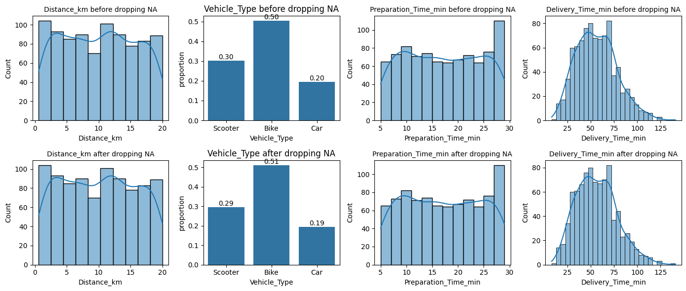
  • Visualize the distribution of the remaining columns before and after dropping the missing values in the chosen column.

  • What do you think is the nature of these missing values (e.g., MCAR, MAR, or MNAR)?

  • Why might this be the case?

---

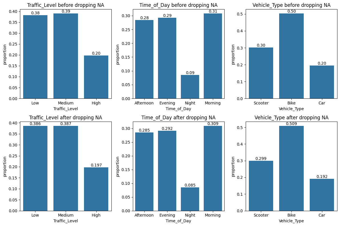
Here we chooe to analyze the missing values of column Weather.

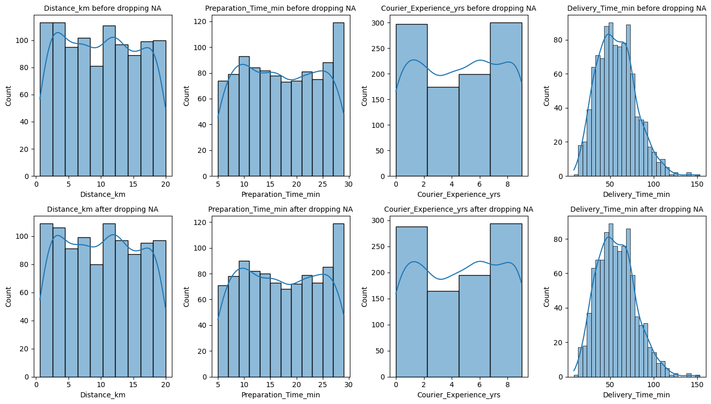
• We analyze the effect of removing missing values on categorical columns, then on numerical columns. This will help us identify the nature of missing values in column Weather.

import matplotlib.pyplot as plt    # for graphs
import seaborn as sns

# Consider weather
# Qualitative columns
qual = data.select_dtypes(include=['object']).columns
fig, axes = plt.subplots(nrows=2, ncols=3, figsize=(12, 8))
i = 0
for va in qual:
  if va != "Weather":
    # Before removing NA in weather
    sns.countplot(data, x=va, ax=axes[0,i], stat="proportion")
    axes[0,i].set_title(va + ' before dropping NA')
    axes[0,i].bar_label(axes[0,i].containers[0], fmt="%.2f")
    # After removing NA in weather
    sns.countplot(data.dropna(subset=['Weather']), x=va, ax=axes[1,i], stat="proportion")
    axes[1,i].set_title(va + ' after dropping NA')
    axes[1,i].bar_label(axes[1,i].containers[0], fmt="%.3f")
    i = i + 1
plt.tight_layout()
plt.show()

import matplotlib.pyplot as plt    # for graphs
import seaborn as sns

# Quantitative columns
quan = data.select_dtypes(include=['number']).columns
fig, axes = plt.subplots(nrows=4, ncols=4, figsize=(14, 8))
i = 0
for va in quan:
  if va != "Order_ID":
  # Before removing NA in weather
    if va != "Delivery_Time_min":
      width = 2
    else:
      width = 5
    sns.histplot(data, x=va, ax=axes[0,i], binwidth=width, kde=True)
    axes[0,i].set_title(va + ' before dropping NA', fontsize=10)
    # After removing NA in weather
    sns.histplot(data.dropna(subset=['Weather']), x=va, ax=axes[1,i], binwidth=width, kde=True)
    axes[1,i].set_title(va + ' after dropping NA', fontsize=10)
    i = i + 1
plt.tight_layout()
plt.show()

As dropping missing values within column Weather does not affect other columns, we can conclude that the nature of the missing values in Weather are ‘Missing Completely At Random (MCAR)’.

data.isna().sum().to_frame().T/data.shape[0] * 100

	Order_ID	Distance_km	Weather	Traffic_Level	Time_of_Day	Vehicle_Type	Preparation_Time_min	Courier_Experience_yrs	Delivery_Time_min
0	0.0	0.0	3.0	3.0	3.0	0.0	0.0	3.0	0.0

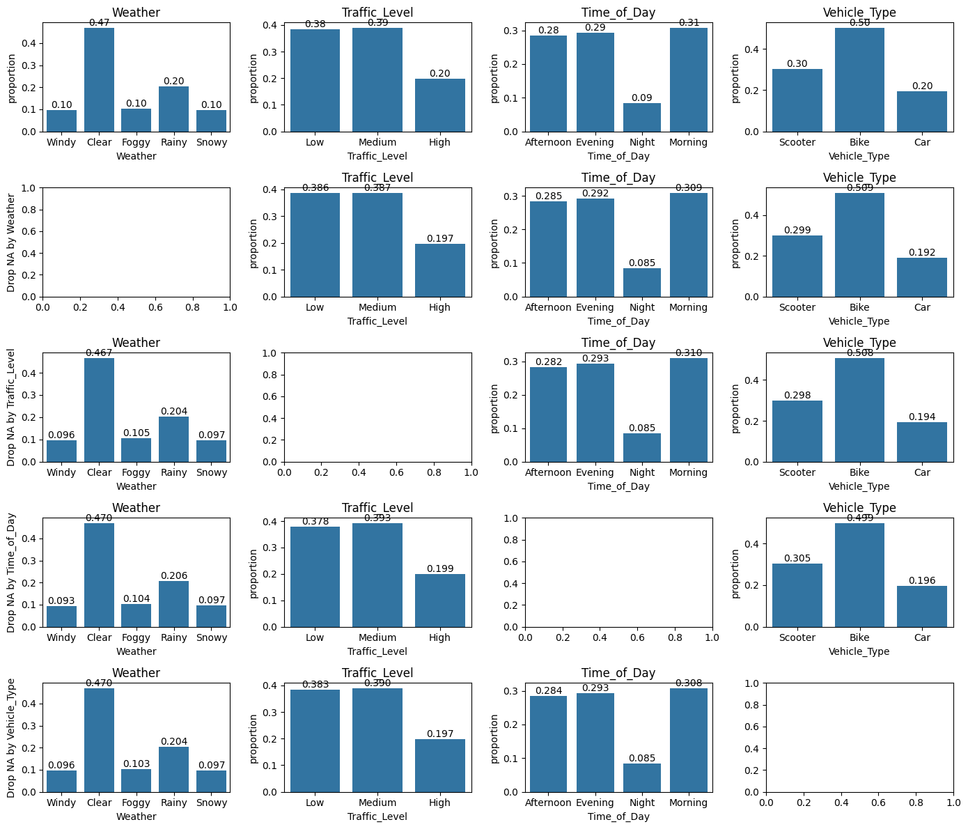
• Repeat the Analysis:

  • Perform the same analysis for other columns with missing values.

We can drop missing values from each variable and consider the distribution of other columns all at once as follows:

# Consider Traffic column
## Qualitative columns

fig, axes = plt.subplots(nrows=5, ncols=4, figsize=(14, 12))
for i, va0 in enumerate(qual):
  sns.countplot(data, x=va0, ax=axes[0,i], stat="proportion")
  axes[0,i].set_title(va0)
  axes[0,i].bar_label(axes[0,i].containers[0], fmt="%.2f")
  axes[i+1,0].set_ylabel(f"Drop NA by {va0}")
  for j, va in enumerate(qual):
      if va != va0:
        sns.countplot(data.dropna(subset=[va0]), x=va, ax=axes[i+1,j], stat="proportion")
        axes[i+1,j].set_title(va)
        axes[i+1,j].bar_label(axes[i+1,j].containers[0], fmt="%.3f")
plt.tight_layout()
plt.show()

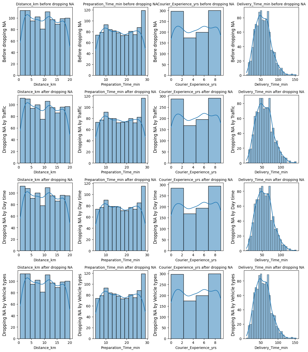
fig, axes = plt.subplots(nrows=4, ncols=4, figsize=(12, 14))
i = 0
for va in quan:
  if va != "Order_ID":
  # Before removing NA
    if va != "Delivery_Time_min":
      width = 2
    else:
      width = 5
    sns.histplot(data, x=va, ax=axes[0,i], binwidth=width, kde=True)
    axes[0,i].set_title(va + ' before dropping NA', fontsize=10)
    axes[0,i].set_ylabel('Before dropping NA', fontsize=12)
    # After removing NA in Traffic level
    sns.histplot(data.dropna(subset=['Traffic_Level']), x=va, ax=axes[1,i], binwidth=width, kde=True)
    axes[1,i].set_title(va + ' after dropping NA', fontsize=10)
    axes[1,i].set_ylabel('Dropping NA by Traffic', fontsize=12)
    # After removing NA in Day time
    sns.histplot(data.dropna(subset=['Time_of_Day']), x=va, ax=axes[2,i], binwidth=width, kde=True)
    axes[2,i].set_title(va + ' after dropping NA', fontsize=10)
    axes[2,i].set_ylabel('Dropping NA by Day time', fontsize=12)
    # After removing NA in Vehicle type
    sns.histplot(data.dropna(subset=['Vehicle_Type']), x=va, ax=axes[3,i], binwidth=width, kde=True)
    axes[3,i].set_title(va + ' after dropping NA', fontsize=10)
    axes[3,i].set_ylabel('Dropping NA by Vehicle types', fontsize=12)
    i = i + 1
plt.tight_layout()
plt.show()

B. Drop all rows with at least one missing values:

• Visualize the distribution of the columns without missing values before and after dropping all rows that contain at least one missing value.

• What observations can you make from these visualizations?

• Impute the missing values using an appropriate method (e.g., mean, median, mode, or advanced imputation techniques).

# Consider weather
# Qualitative columns
quan = data.select_dtypes(include=['number']).columns
fig, axes = plt.subplots(nrows=2, ncols=4, figsize=(14, 6))
i = 0
for va in ['Distance_km', 'Vehicle_Type', 'Preparation_Time_min', 'Delivery_Time_min']:
    if va == "Vehicle_Type":
      sns.countplot(data, x=va, ax=axes[0,i], stat="proportion")
      axes[0,i].set_title(va + ' before dropping NA')
      axes[0,i].bar_label(axes[0,i].containers[0], fmt="%.2f")
      # After removing NA in weather
      sns.countplot(data.dropna(), x=va, ax=axes[1,i], stat="proportion")
      axes[1,i].set_title(va + ' after dropping NA')
      axes[1,i].bar_label(axes[1,i].containers[0], fmt="%.2f")
    else:
      if va != "Delivery_Time_min":
        width = 2
      else:
        width = 5
      sns.histplot(data.dropna(), x=va, ax=axes[0,i], binwidth=width, kde=True)
      axes[0,i].set_title(va + ' before dropping NA', fontsize=10)

      # After removing NA in weather
      sns.histplot(data.dropna(), x=va, ax=axes[1,i], binwidth=width, kde=True)
      axes[1,i].set_title(va + ' after dropping NA', fontsize=10)
    i = i + 1
plt.tight_layout()
plt.show()

• Before and after dropping the missing values, the distributions of columns are mostly preserved, therefore they are missing completely at random. Dropping or imputing with mean or median or mode is fine.

C. Analyzing Connections Between Columns

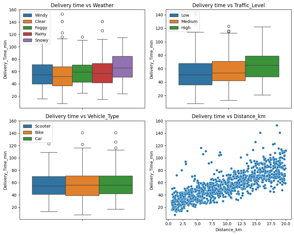
• Impact of Weather on Delivery Time: determine if weather conditions affect delivery time.

• Influence of Traffic Level: determine whether traffic levels impact delivery time?

• Effect of Vehicle Type: How can we evaluate if the type of vehicle used influences delivery time?

• Role of Distance: How can we analyze the relationship between distance and delivery time?

fig, axs = plt.subplots(nrows=2, ncols=2, figsize=(10, 8))
for i, va in enumerate(["Weather", "Traffic_Level", "Vehicle_Type", "Distance_km"]):
    if va != "Distance_km":
        sns.boxplot(data, y="Delivery_Time_min", hue=va, ax=axs[i//2, i%2])
        axs[i//2, i%2].legend(loc="upper left")
    else:
        sns.scatterplot(data, x=va, y="Delivery_Time_min", ax=axs[i//2, i%2])
    axs[i//2, i%2].set_title(f"Delivery time vs {va}")
plt.tight_layout()
plt.show()

According to the previous graphs:

• Weahter condition seems to not affect delivery time that much except for the snowy time where the delivery times take slightly longer than other conditions.
• The traffic level also seems to not influence delivery time that much either. The more busy the traffic, the slightly longer delivery time.
• The vehicle type on the other hand does not influence the delivery time at all since the boxplots look nearly identical on all types of vehicle.
• The Scatterplot shows a clear trend incating that the longer the distance, the longer time it takes to delivery the foods.

2. Auto-MPG Dataset

This dataset contains spec of various cars and is available in kaggle. For more, read here.

import kagglehub

# Download latest version
path = kagglehub.dataset_download("uciml/autompg-dataset")
auto = pd.read_csv(path + '/auto-mpg.csv')
auto.head()

• Investigate factors that may affect the quality of the dataset and implement appropriate measures to handle them.

Further Reading

• Pandas python library: https://pandas.pydata.org/docs/getting_started/index.html#getting-started

• Pandas Cheatsheet: https://pandas.pydata.org/Pandas_Cheat_Sheet.pdf

• 10 Minute to Pandas: https://pandas.pydata.org/docs/user_guide/10min.html

• Some Pandas Lession: https://www.kaggle.com/learn/pandas