Hypothesis Testing
z-test & t-test
INF-604: Data Analysis
![]()
Motivation Example
Newborn baby weights
The weight of new born babies is an important
indicator for the baby’s health.Assumption: Newborn babies who weigh more
than the average weight of newborns are considered healthy.
Tell me, what should I do to check if my newborn brother is healthy?

Motivation Example
Newborn baby weights
- We should first estimate the average weight of newborn babies.
- A collected sample of size \(n=100\) gives \(\overline{W}=3.5\) kg.
- We don’t know the true healthy weight. Can we trust this estimate?
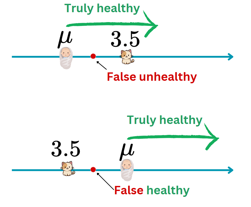
- If \(\mu\) is the true mean of baby weight, there’re 2 problems:
- If \(\mu < 3.5\), healthy babies may be considered unhealthy.
- If \(\mu > 3.5\), unhealthy babies may be considered healthy.
- One of these two mistakes is much much more important than another! Which one? Call it Type I Mistake, and we must control it!
:::
Motivation Example
Hypothesis setting and goal
- In this case, we want to build a decision rule that
- Judges babies based on the estimate \(\overline{W}=3.5\) and
- Controls the risk of committing Type I Mistake to be small.
- Here is the corresponding hypothesis test: \[\begin{cases}\color{red}{H_0}:\mu\geq 3.5\\ \color{green}{H_1}: \mu<3.5,\end{cases}\] where
- \(\color{red}{H_0}:\) Null hypothesis to be rejected with low risk of comitting Type I Mistake.
- \(\color{green}{H_1}:\) Alternative hypothesis to be supported.

Probability
Probability on a fintie set
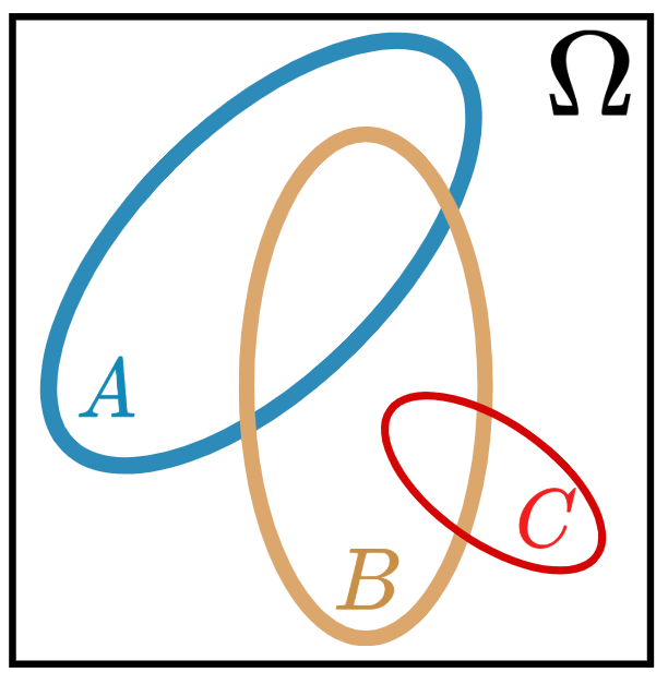
- Probabilty on a finite set: if \(A\subset \Omega\) then \(\color{blue}{\mathbb{P}(A)=\frac{n(A)}{n(\Omega)}}.\)
- Previous example: Coin toss (H and T) 3 times:
- Sample space: \(n(\Omega)=8\).
- Probability:
- A: “Head came out twice”, \(\mathbb{P}(A)=3/8\).
- B: “No head before tails”, \(\mathbb{P}(B)=3/8\).
- C: “Number of heads and tails are equal”, \(\mathbb{P}(C)=0\).
Probability
Axioms of probability
- Probability satisfies the following 3 axioms:
- \(\mathbb{P}(A)\geq 0\) for all \(A\subset \Omega\).
- \(\mathbb{P}(\Omega)=1\).
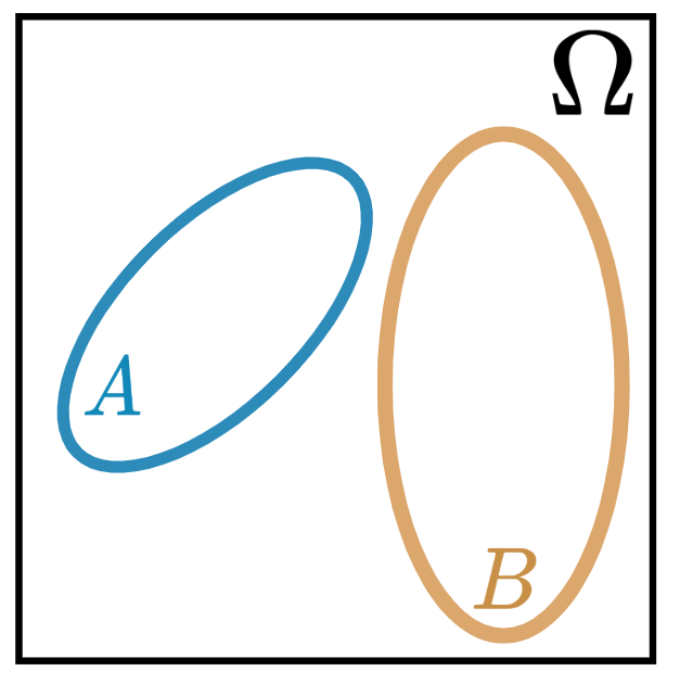
- If \(A,B\subset\Omega\) are two disjoint events, then \[\mathbb{P}(A\cup B)=\mathbb{P}(A)+\mathbb{P}(B).\]
- Theorem: \(\color{blue}{A,B\subset\Omega: \mathbb{P}(A\cup B)=\mathbb{P}(A)+\mathbb{P}(B)-\mathbb{P}(A\cap B)}.\)
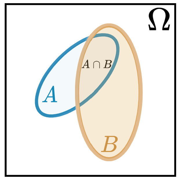
- Our example: \(\mathbb{P}(A\cup B)=\mathbb{P}(A)+\mathbb{P}(B)-\mathbb{P}(A\cap B)=3/8+3/8-1/8=5/8\).
Probability
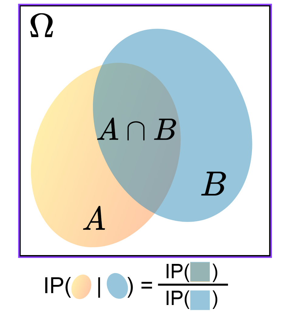
Conditional Probability & Independency
- If \(A,B\subset \Omega:\) with \(\mathbb{P}(B)>0\), the conditional probability of \(A\) given \(B\) is defined by: \[\color{blue}{\mathbb{P}(A|B)=\frac{\mathbb{P}(A\cap B)}{\mathbb{P}(B)}=\frac{n(A\cap B)}{n(B)}}.\]
- Example: \(\mathbb{P}(A|B)=\frac{1/8}{3/8}=1/3\).
- An event \(A\) is independent of \(B\), denoted by \(A\perp B\) if and only if: \[\color{blue}{\mathbb{P}(A|B)=\mathbb{P}(A)}.\]
Probability
Expectation & variance of DRV
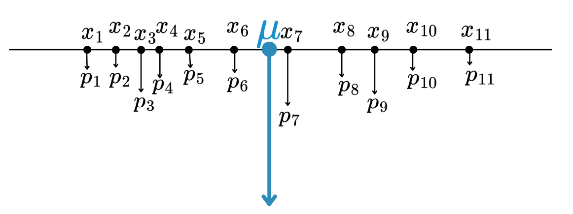
- If \(X\) is a discrete random variable taking values in \(\{x_1,x_2,\dots,x_n\}\)
- The Expectation of \(X\): \[\mu=\mathbb{E}(X)=\sum_{k=1}^{n}x_kp_k.\]
- The Variance of \(X\): \[\sigma^2=\mathbb{V}(x)=\sum_{k=1}^np_k(x_k-\mu)^2.\]
- Our example: \(X\) = Number of heads: \[\begin{align*}\mathbb{E}(X)&=\sum_{k=1}^{n}x_kp_k\\ &=0(1/8)+1(3/8)+2(3/8)+3(1/8)=1.5\\ \mathbb{V}(X)&=\sum_{k=1}^{n}p_k(x_n-1.5)^2\\ &=(0-1.5)^2(1/8)+(1-1.5)^2(3/8)+(2-1.5)^2(3/8)\\ &+(3-1.5)^2(1/8)=0.75.\end{align*}\]
Probability
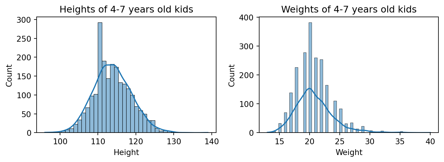
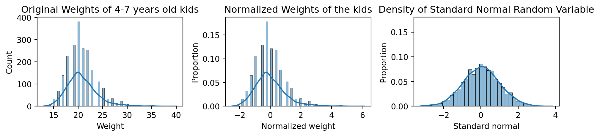
Normal/Gaussian Random Variable
- Consider our French kid dataset:
| Gender | Age | Height | Weight | |
|---|---|---|---|---|
| 1 | M | 74 | 116 | 18 |
| 2 | M | 69 | 120 | 23 |
| 3 | M | 72 | 121 | 25 |
Probability
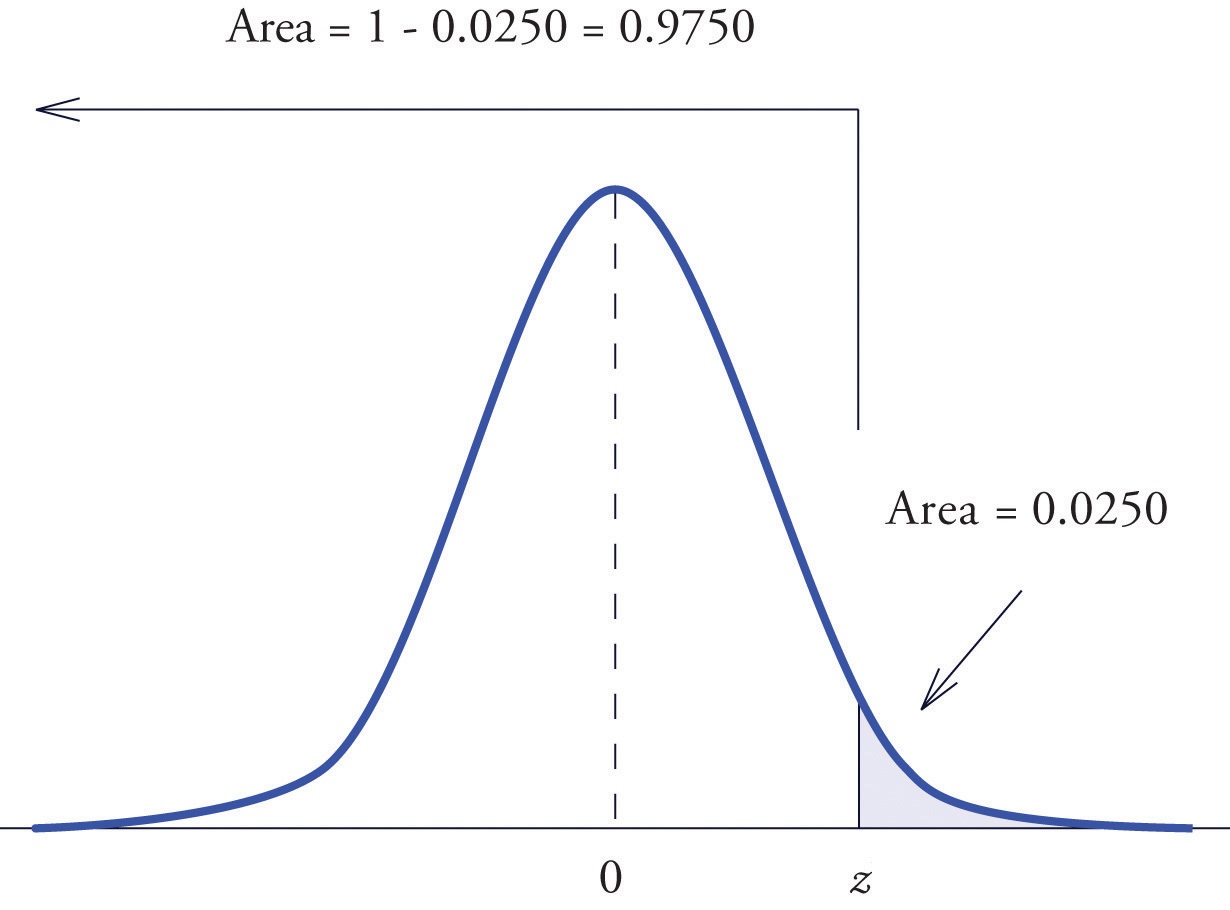
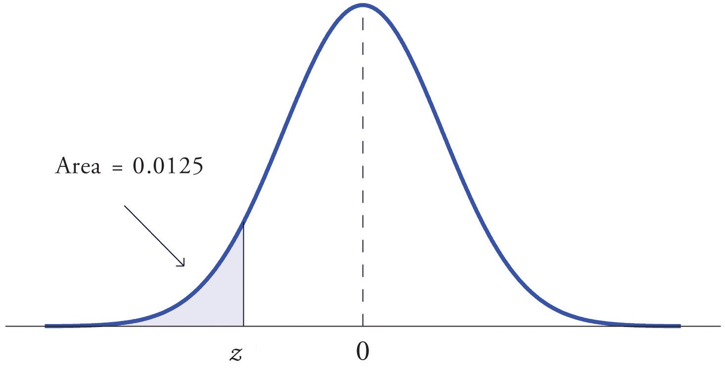
Standard Normal & Property
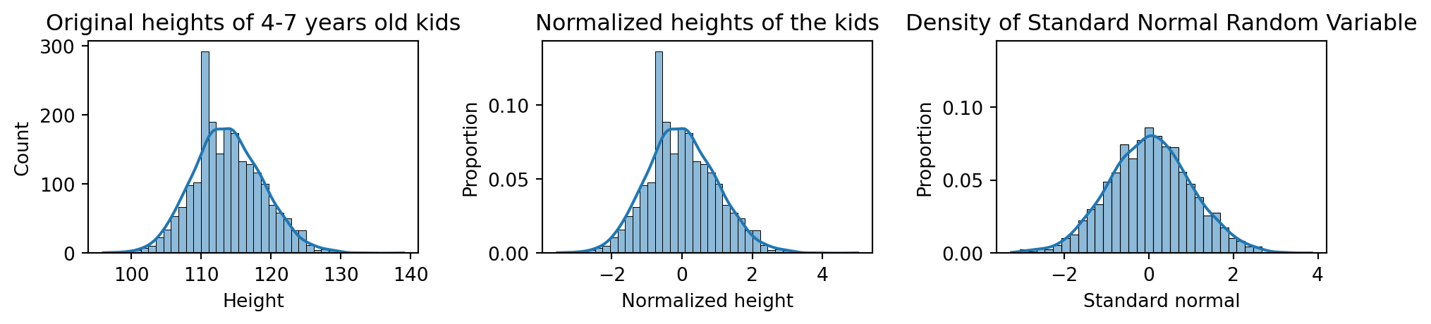
Probability
Standard Normal & Property

And now, we have enough probability tools!
z-Test
Z-statistics and Rejection Region
Z-test statistics & Rejection Region
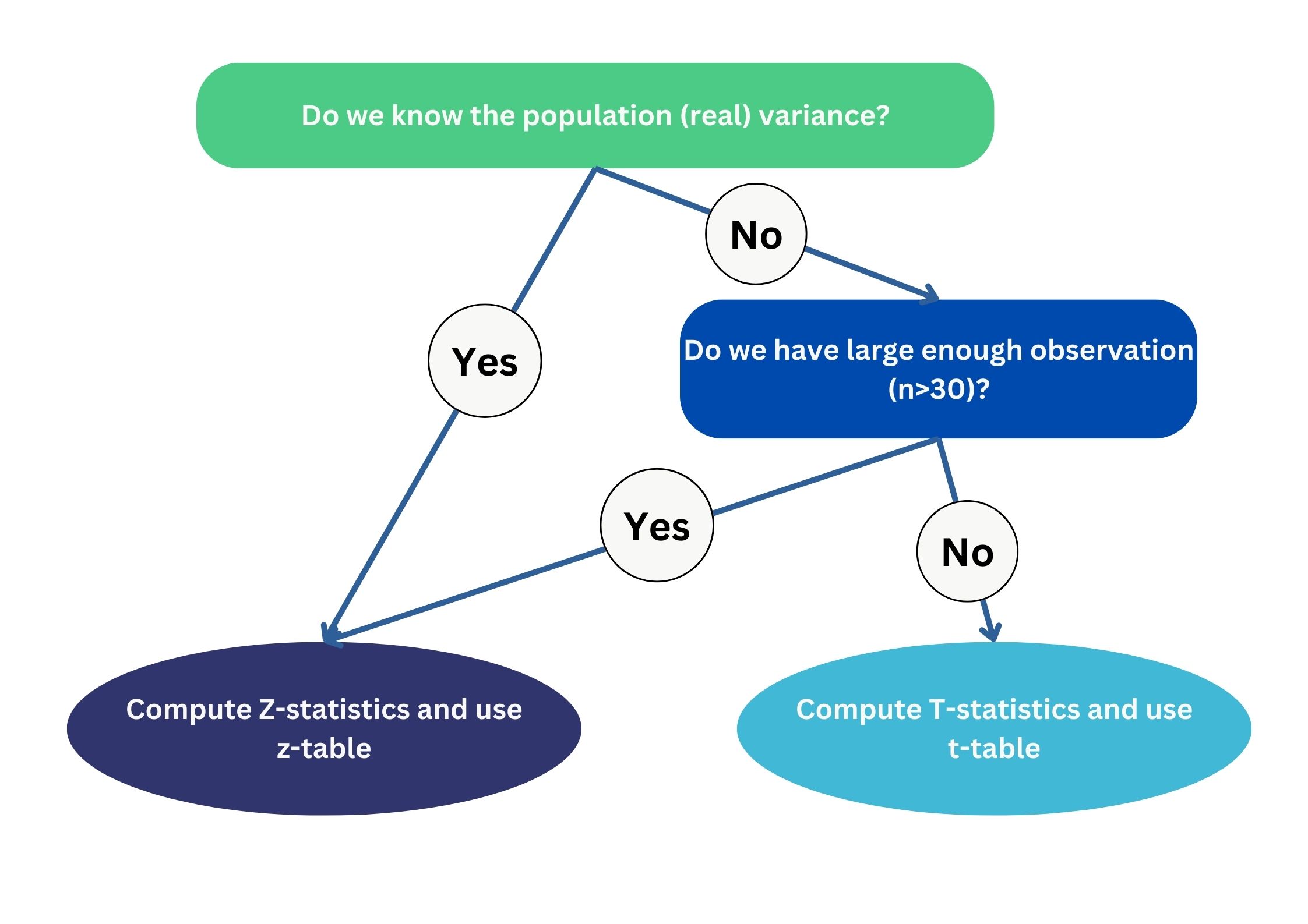
- Key assumption: Assume that \(X_1,\dots,X_n\sim{\cal N}(\mu, \sigma^2)\) are iid with an unknown mean \(\mu\) and a known standard deviation \(\sigma>0\).
- If \(H_0\) is True, then for any \(\color{red}{\alpha}\in (0,1)\) we have
- The quantity: \(Z=\frac{\overline{X}_n-\color{blue}{\mu_0}}{\sigma/\sqrt{n}}\sim{\cal N}(0,1)\) “z-value”.
- If we choose \(\color{red}{z_{\alpha}}\) such that \(\mathbb{P}(Z>\color{red}{z_{\alpha}})=\color{red}{\alpha}\), then “if we reject \(H_0\) whenever \(Z>\color{red}{z_{\alpha}}\), it’s guaranteed that” \[\mathbb{P}(\color{red}{\text{Type I Error}})=\mathbb{P}(\color{red}{\text{Reject }}H_0|H_0\color{blue}{\text{ is True}})=\color{red}{\alpha}.\]
- The set of \(\color{red}{R(\alpha)=\{z: z>z_{\alpha}\}}\) is called Rejection Region at level \(\alpha\), meaning that if \(Z\in\color{red}{R(\alpha)}\), we can reject \(H_0\) with confidence level \(1-\color{red}{\alpha}\).
z-Test
Z-test Summary for (\(S_>\), one-tailed)
Z-test Summary (\(S_>\))
- Suppose the sample: \(X_1,\dots,X_n\sim{\cal N}(\mu,\sigma^2)\) with known \(\sigma^2\) and unknown \(\mu\).
- For some \(\color{blue}{\mu_0}\) given, to test \(H_0:\mu=\color{blue}{\mu_0}\) against \(H_1:\mu>\color{blue}{\mu_0}\) we do:
- Compute \(Z=\frac{\overline{X}_n-\color{blue}{\mu_0}}{\sigma/\sqrt{n}}\)
- For a given significance level \(\color{red}{\alpha}\), compute \(\color{red}{z_\alpha}\) such that \(\mathbb{P}(Z\geq\color{red}{z_\alpha})=\color{red}{\alpha}\).
- Decision:
- If \(Z\geq\color{red}{z_\alpha}\), we reject \(H_0\) with confidence level \(1-\color{red}{\alpha}\).
- If \(Z< \color{red}{z_\alpha}\), we CANNOT \(H_0\) due to insufficient evidence.
z-Test
Z-test Summary for (\(S_<\), one-tailed)
Z-test Summary (\(S_<\))
- Suppose the sample: \(X_1,\dots,X_n\sim{\cal N}(\mu,\sigma^2)\) with known \(\sigma^2\) and unknown \(\mu\).
- For some \(\color{blue}{\mu_0}\) given, to test \(H_0:\mu=\color{blue}{\mu_0}\) against \(H_1:\mu<\color{blue}{\mu_0}\) we do:
- Compute \(Z=\frac{\overline{X}_n-\color{blue}{\mu_0}}{\sigma/\sqrt{n}}\)
- For a given significance level \(\color{red}{\alpha}\), compute \(\color{red}{z_\alpha}\) such that \(\mathbb{P}(Z\leq\color{red}{z_\alpha})=\color{red}{\alpha}\).
- Decision:
- If \(Z\leq\color{red}{z_\alpha}\), we reject \(H_0\) with confidence level \(1-\color{red}{\alpha}\).
- If \(Z> \color{red}{z_\alpha}\), we CANNOT reject \(H_0\) due to insufficient evidence.
- Ex: (Baby weight) Test \(H_0:\mu=3.75\) against \(H_1:\mu<3.75\) at \(\alpha=0.05\), knowing that \(\sigma=0.5\) kg and \(\overline{W}=3.5\) kg (assuming that baby weights are normally distributed). How about when \(\overline{W}=2.9\) kg?
z-Test
Z-test Summary for (\(S_\neq\) Two-tailed)
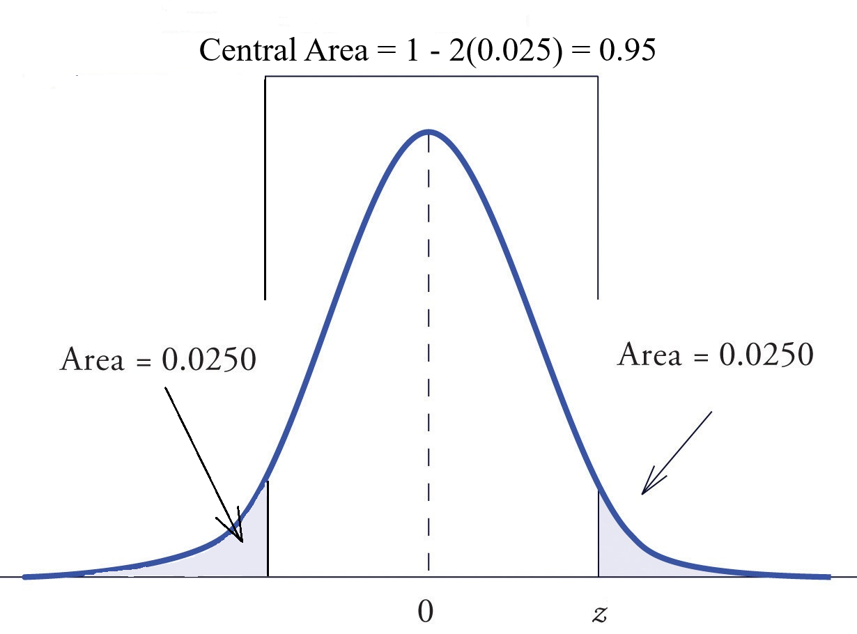
Z-test Summary (\(S_\neq\), two-sided test)
- Suppose the sample: \(X_1,\dots,X_n\sim{\cal N}(\mu,\sigma^2)\) with known \(\sigma^2\) and unknown \(\mu\).
- For some \(\color{blue}{\mu_0}\) given, to test \(H_0:\mu=\color{blue}{\mu_0}\) against \(H_1:\mu\neq\color{blue}{\mu_0}\) we do:
- Compute \(Z=\frac{\overline{X}_n-\color{blue}{\mu_0}}{\sigma/\sqrt{n}}\)
- For a given significance level \(\color{red}{\alpha}\), compute \(\color{red}{z_{\alpha/2}}\) such that \(\mathbb{P}(|Z|\geq\color{red}{z_{\alpha/2}})=\color{red}{\alpha}\).
- Decision:
- If \(|Z|\geq\color{red}{z_{\alpha/2}}\), we reject \(H_0\) with confidence level \(1-\color{red}{\alpha}\).
- If \(|Z|< \color{red}{z_{\alpha/2}}\), we CANNOT reject \(H_0\) due to insufficient evidence.
z-Test
Example: Newborn weights in France, 2016
- Test \(\color{red}{\mu=3}\) kg against \(\color{green}{\mu\neq 3}\) kg at significance level \(\alpha=0.1\), given that \(n=745000,\overline{X}_n=3.25\) and \(\sigma^2=1.5\). How about with \(\color{blue}{\mu_0=3.75}\)?
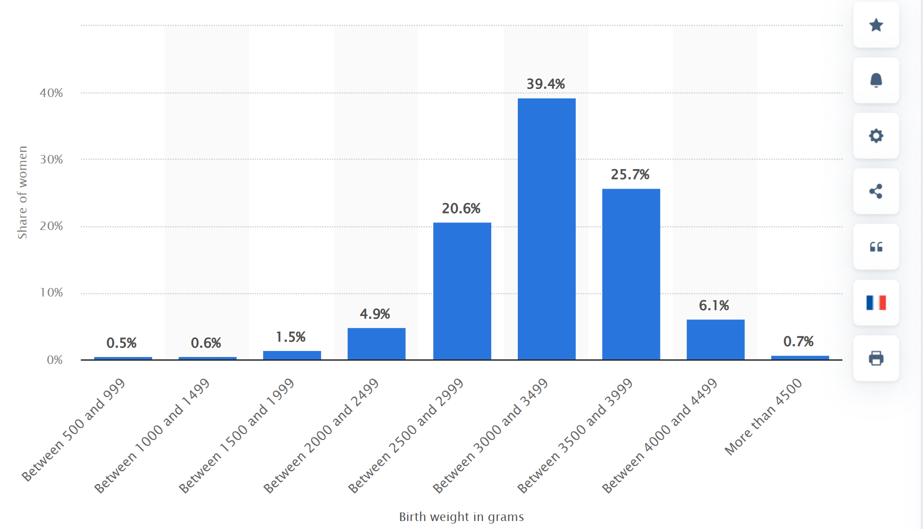
Source: Birth weight of newborns delivered in France 2016, Statistia.
t-Test
\(t\)-Table for (\(T_>\) one-tailed)
- When \(n\) is small (\(<30\)) and \(\sigma>0\) is unknown, we use \(t\)-distribution.
\(t\)-Test Summary (\(T_>\))
- Suppose the sample: \(X_1,\dots,X_n\sim{\cal N}(\mu,\color{red}{\sigma^2})\) with unknown \(\mu\) and \(\color{red}{\sigma^2}\).
- For some \(\color{blue}{\mu_0}\) given, to test \(H_0:\mu={\mu_0}\) against \(H_1:\mu>\color{blue}{\mu_0}\) we do:
- Compute \(\color{red}{\hat{\sigma}^2=\frac{1}{n-1}\sum_{i=1}^n(X_i-\overline{X}_n)^2}\) (estimator of \(\color{red}{\sigma^2}\)), then \(T=\frac{\overline{X}_n-\color{blue}{\mu_0}}{\color{red}{\hat{\sigma}}/\sqrt{n}}\)
- For a given significance level \(\color{red}{\alpha}\), compute \(\color{red}{t_\alpha}\) such that \(\mathbb{P}(T\geq\color{red}{t_\alpha})=\color{red}{\alpha}\).
- Decision:
- If \(T\geq\color{red}{t_\alpha}\), we reject \(H_0\) with confidence level \(1-\color{red}{\alpha}\).
- If \(T< \color{red}{t_\alpha}\), we CANNOT \(H_0\) due to insufficient evidence.
t-Test
\(t\)-Table for (\(T_<\) one-tailed)
\(t\)-Test Summary (\(T_<\))
- Suppose the sample: \(X_1,\dots,X_n\sim{\cal N}(\mu,\color{red}{\sigma^2})\) with unknown \(\mu\) and \(\color{red}{\sigma^2}\).
- For some \(\color{blue}{\mu_0}\) given, to test \(H_0:\mu={\mu_0}\) against \(H_1:\mu<\color{blue}{\mu_0}\) we do:
- Compute \(\color{red}{\hat{\sigma}^2=\frac{1}{n-1}\sum_{i=1}^n(X_i-\overline{X}_n)^2}\) (estimator of \(\color{red}{\sigma^2}\)), then \(T=\frac{\overline{X}_n-\color{blue}{\mu_0}}{\color{red}{\hat{\sigma}}/\sqrt{n}}\)
- For a given significance level \(\color{red}{\alpha}\), compute \(\color{red}{t_\alpha}\) such that \(\mathbb{P}(T\leq\color{red}{t_\alpha})=\color{red}{\alpha}\).
- Decision:
- If \(T\leq\color{red}{t_\alpha}\), we reject \(H_0\) with confidence level \(1-\color{red}{\alpha}\).
- If \(T> \color{red}{t_\alpha}\), we CANNOT \(H_0\) due to insufficient evidence.
t-Test
\(t\)-Table for (\(T_{\neq}\) two-tailed)
\(t\)-Test Summary (\(T_\neq\))
- Suppose the sample: \(X_1,\dots,X_n\sim{\cal N}(\mu,\color{red}{\sigma^2})\) with unknown \(\mu\) and \(\color{red}{\sigma^2}\).
- For some \(\color{blue}{\mu_0}\) given, to test \(H_0:\mu={\mu_0}\) against \(H_1:\mu\neq\color{blue}{\mu_0}\) we do:
- Compute \(\color{red}{\hat{\sigma}^2=\frac{1}{n-1}\sum_{i=1}^n(X_i-\overline{X}_n)^2}\) (estimator of \(\color{red}{\sigma^2}\)), then \(T=\frac{\overline{X}_n-\color{blue}{\mu_0}}{\color{red}{\hat{\sigma}}/\sqrt{n}}\).
- For a given significance level \(\color{red}{\alpha}\), compute \(\color{red}{t_\alpha}\) such that \(\mathbb{P}(|T|\geq\color{red}{t_\alpha})=\color{red}{\alpha}\).
- Decision:
- If \(|T|\geq \color{red}{t_\alpha}\), we reject \(H_0\) with confidence level \(1-\color{red}{\alpha}\).
- If \(|T|< \color{red}{t_\alpha}\), we CANNOT \(H_0\) due to insufficient evidence.
Summary
![]()