Exploratory Data Analysis (EDA): Correlation Analysis


INF-604: Data Analysis

Lecturer: Dr. Sothea HAS

Outline

  • Motivation

  • Pearson Correlation Coefficient

  • Spearman’s Rank Correlation Coefficient

  • \(\eta\)-squared Coefficient

Motivation

Motivation

Consider Gapminder Dataset (1704, 5)

  • In 2007, we observed that
    • People in countries with strong economies appeared to be healthier.
    • The economy and health conditions did not seem to be related to population size.
Code
import plotly.graph_objects as go
import numpy as np
import plotly.express as px
from gapminder import gapminder
data2007 = gapminder.query("year == 2007")
fig1 = px.scatter(
    data2007, x="gdpPercap", y="lifeExp", 
    hover_name="country", opacity=0.7,
    log_x=True)
fig1.update_traces(marker=dict(size=10))
fig1.update_layout(height=310, width=500, title="The world GDP vs (log) LifeExp in 2007")
fig1.show()
Code
data2007 = gapminder.query("year == 2007")
fig2 = px.scatter(
    data2007, x="gdpPercap", y="pop", 
    hover_name="country", opacity=0.7,
    log_x=True, log_y=True)
fig2.update_traces(marker=dict(size=10))
fig2.update_layout(height=310, width=500, title="The world GDP vs (log) Population in 2007")
fig2.show()

Motivation

Consider Gapminder Dataset (1704, 5)

  • In 2007, we also saw that
    • Life expectancy and GDP per capita varied across different continents.
Code
sorted_data = data2007.sort_values(by='lifeExp')
fig3 = px.box(
    data2007, x="continent", y="lifeExp", 
    hover_name="country", color="continent", 
    category_orders={'continent': sorted_data['continent']})
fig3.update_layout(title="Life expectancy on each continent in 2007", height=350, width=500)
fig3.show()
Code
sorted_data = data2007.sort_values(by='gdpPercap')
fig4 = px.box(
    data2007, x="continent", y="gdpPercap", 
    hover_name="country", color="continent", 
    category_orders={'continent': sorted_data['continent']})
fig4.update_layout(title="GDP per Capita on each continent in 2007", height=350, width=500)
fig4.show()

Motivation

Consider Gapminder Dataset (1704, 5)


We have explored how to summarize, visualized a single column and relationship between many columns.

We will now explore some indicators that capture/summarize such tendency or relationship.

Summary/Figure \(\color{red}{\underset{\text{Visualization}}{\longleftarrow}}\) Data

Summary/Figure \(\color{red}{\underset{\text{Visualization}}{\longleftarrow}}\) Data \(\color{blue}{\underset{\text{Correlation}}{\longrightarrow}}\) Indicator.

Motivation

Consider Gapminder Dataset (1704, 5)


Pearson Correlation Coefficient

Pearson Correlation Coefficient

Covariance between two Quan. columns

  • Suppose \(X=[\text{x}_1,\text{x}_2,...,\text{x}_n]\) be a quan. column.
  • Mean/average: \(\overline{\text{x}}=\displaystyle\frac{1}{n}\sum_{i=1}\text{x}_i\).
  • Variance: \(V(X)=\displaystyle\frac{1}{n-1}\sum_{i=1}^n(\text{x}_i-\overline{x})^2.\)
  • Standard deviation: \(s=\sqrt{V(X)}\).
  • If \(Y=[\text{y}_1,\text{y}_2,\dots,\text{y}_n]\) is an other quan. column, the covaraince between \(X\) and \(Y\) is defined by

\[\text{Cov}(X,Y)=\frac{1}{n-1}\sum_{i=1}(\text{x}_i-\overline{x})(\text{y}_i-\overline{y}).\]

Code
df = px.data.tips()
fig = px.scatter(df, y="tip", x="total_bill", color="sex", hover_data=df.columns)
fig.update_layout(width=380, height=300, title="Tips vs total bill & gender")
fig.show()
tip total_bill sex
0 1.01 16.99 Female
1 1.66 10.34 Male
2 3.50 21.01 Male

Pearson Correlation Coefficient

Covariance between two Quan. columns

  • Covariance between quan. columns \(X\) and \(Y\):

\[\text{Cov}(X,Y)=\frac{1}{n-1}\sum_{i=1}(\text{x}_i-\overline{x})(\text{y}_i-\overline{y}).\]

  • It determines tendency/direction of the relationship between the two variables.
    • Positive value \(\approx\) change in the same direction.
    • Negative value \(\approx\) change in opposite direction.

It’s hard to interpret the value of covariance as it can be large or small according to the scale of \(X\) and \(Y\).

Code
fig.update_layout(title=f"Tips vs total bill (Cov = {float(np.cov(df['tip'].values, df['total_bill'].values).round(2)[0,1])}) & gender ")
fig.show()
tip total_bill sex
0 1.01 16.99 Female
1 1.66 10.34 Male
2 3.50 21.01 Male

Pearson Correlation Coefficient

Definition

Pearson correlation coefficient

  • Correlation between two quan. columns \(X\) and \(Y\): \[r=r_{X,Y}=\frac{\sum_{i=1}^n(\text{x}_{i}-\overline{x})(\text{y}_{i}-\overline{y})}{\sqrt{\left(\sum_{i=1}^n(x_{i1}-\overline{x}_{1})^2\right)\left(\sum_{i=1}^n(x_{i2}-\overline{x}_{2})^2\right)}}=\frac{\text{Cov}(X,Y)}{s_Xs_Y}.\]
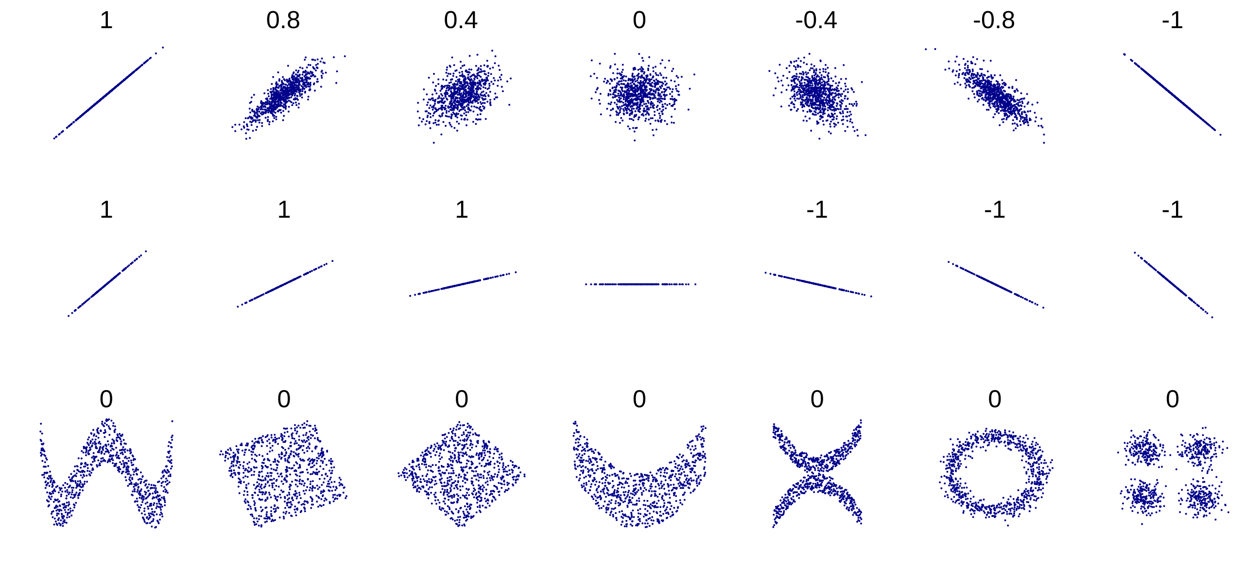
  • It quantifies the linear relationship/tendency between the two variables.
    • For any pair \(X\) and \(Y\) one has \(-1\leq r\leq 1\).
    • If \(r\approx 1\), then \(X\) and \(Y\) are positively correlated (change in the same direction).
    • If \(r\approx -1\), then \(X\) and \(Y\) are negatively correlated (change in opposite direction).
    • If \(r\approx 0\), then \(Y\) and \(Y\) are decorrelated (no pattern/trend/tendency).
  • It helps identifying informative/useful inputs for the building models.
  • It also helps identifying redundant (strongly correlated) inputs.
  • For tip example: \(\text{Corr}(\text{tip}, \text{bill})=\) 0.676.
  • Note: Correlation does not imply causation; it only indicates a relationship, not a cause-and-effect link [👉 For more, read here].

Pearson Correlation Coefficient

Examples:

Pearson Correlation Coefficient

Correlation matrix: Gapinder

  • Consider Pearson cor. on Gapminder in 2007:
cor = data2007[["gdpPercap", "lifeExp", "pop"]].corr()
cor.style.background_gradient(cmap='Accent')
  gdpPercap lifeExp pop
gdpPercap 1.000000 0.678662 -0.055676
lifeExp 0.678662 1.000000 0.047553
pop -0.055676 0.047553 1.000000


Pearson Correlation Coefficient

Summary

  • Pearson correlation coefficient measures linear relationship between two quan. columns.

  • It captures the pattern of the scatterplot between the two columns.

  • It only describes the tendency but not cause-and-effect relation.

  • The correlation may not be reliable when/with:

    • There are outliers
    • Small number of observations
    • Non-linear relation and confounding variables…

Spearman’s Rank Correlation

Spearman’s Rank Correlation

Beyond linearity

  • Pearson correlation is sensitive to outliers (we will see that in the lab) and cannot capture non-linear relationship between quantitaive columns.
  • It is not sutiable for ordinal data (dislike-like rating, for example).
  • Spearman’s Rank Correlation does not rely on the value of observations but rather depends on the ‘rank’ of the observations.
  • Let \(R[\text{x}_i]\) and \(R[\text{y}_i]\) be the rank of observations \(\text{x}_i\) and \(\text{y}_i\) in their own list, then Spearman’s rank correlation coefficient between \(X\) and \(Y\) is defined as the Pearson correlation over the rank of \(X\) and \(Y\), i.e., \[\rho_{X,Y}=r_{R[X],R[Y]}=\frac{\text{Cov}(R[X],R[Y])}{s_{R[X]},s_{R[Y]}}=1-\frac{6\sum_{i=1}^nd_i^2}{n(n^2-1)},\] where \(d_i=R[\text{x}_i]-R[\text{y}_i]\) be the distance in rank of observation \(i\)-th.

Spearman’s Rank Correlation

Example

  • Example: \(X=[3,2,1,5,8]\) and \(Y=[8,5,0,23,80]\)

Pearson

  • \(\overline{x}=\frac{3+2+1+5+9}{5}=\color{red}{4}\) and \(\overline{y}=\frac{8+5+0+23+80}{5}=\color{blue}{23.2}\).
  • \(s_X=\sqrt{\frac{(3-\color{red}{4})^2+(2-\color{red}{4})^2+\dots+(8-\color{red}{4})^2}{n-1}}=2.8284\) and \(s_Y=\sqrt{\frac{(8-\color{blue}{23.2})^2+(5-\color{blue}{23.2})^2+\dots+(80-\color{blue}{23.2})^2}{n-1}}=29.417\).
  • \(r_{X,Y}=\frac{(3-\color{red}{4})(8-\color{blue}{23.2})+\dots+(8-\color{red}{4})(80-\color{blue}{23.2})}{(2.8284)(29.417)}=0.9735.\)

Spearman

  • \(R[X]=[3,2,1,4,5]\) and \(R[Y]=[3,2,1,4,5]\).
  • All \(d_i=0\) therefore \(\rho_{X,Y}=1-\frac{6\sum_{i}d_i^2}{5(5^2-1)}=1\).

Spearman’s Rank Correlation

Correlation matrix: Gapinder

  • Consider Pearson cor. on Gapminder in 2007:
cor = data2007[["gdpPercap", "lifeExp", "pop"]].corr()
cor.style.background_gradient(cmap='Accent')
  gdpPercap lifeExp pop
gdpPercap 1.000000 0.678662 -0.055676
lifeExp 0.678662 1.000000 0.047553
pop -0.055676 0.047553 1.000000
  • Consider Spearman cor. on Gapminder in 2007:
cor = data2007[["gdpPercap", "lifeExp", "pop"]]\
    .corr("spearman")
cor.style.background_gradient(cmap='Accent')
  gdpPercap lifeExp pop
gdpPercap 1.000000 0.856590 -0.064588
lifeExp 0.856590 1.000000 0.003355
pop -0.064588 0.003355 1.000000

Spearman’s Rank Correlation

More example

Spearman’s Rank Correlation

Summary

Aspect Pearson Spearman
Type Parametric Non-parametric
Measure Linear relationship Monotonic relationship
Data Type Continuous Ordinal or continuous
Outliers Sensitive to outliers Less sensitive to outliers
Range -1 to 1 -1 to 1
Interpretation \(\bullet\) 1: Perfect positive linear relationship
\(\bullet\) -1: Perfect negative linear relationship
\(\bullet\) 0: No linear relationship
\(\bullet\) 1: Perfect positive rank correlation
\(\bullet\) -1: Perfect negative rank correlation
\(\bullet\) 0: No rank or no monotonicity correlation

\(\eta\)-squared Coefficient

\(\eta\)-squared Coefficient

quan.-qualitative

Code
data2007[['continent', 'lifeExp', 'gdpPercap']].head(4)
continent lifeExp gdpPercap
11 Asia 43.828 974.580338
23 Europe 76.423 5937.029526
35 Africa 72.301 6223.367465
47 Africa 42.731 4797.231267
  • Recall that in 2007:
    • continent and lifeExp are related (life expectancy varies across different continents).
    • gdpPercap also differs across different continents.
  • How can we quantify these relations?

\(\eta\)-squared Coefficient

quan.-qualitative

  • If \(G\) and \(X\) are qualitative and quan. columns resp.
  • Between Sum of Squares (BSS): \[\color{blue}{\text{BSS}}=\sum_{g=1}^Gn_g(\overline{\text{x}}_g-\color{blue}{\overline{\text{x}}})^2,\] where
    • \(\overline{\text{x}}_g\) is the mean of \(X\) over a category \(g\) of \(G\).
    • \(\color{blue}{\overline{\text{x}}}\) is the global mean of \(X\).
    • \(n_g\) is the number of observations within category \(g\) of \(G\).
  • It measures how distant the values of \(X\) are across different groups of \(G\).
  • Total Sum of Squares (TSS): \[\color{red}{\text{TSS}}=\sum_{i=1}^n(\text{x}_i-\color{blue}{\overline{\text{x}}})^2.\]

\(\eta\)-squared Coefficient

quan.-qualitative

  • \(\eta\)-squared coefficient: \(\eta^2=\frac{\color{blue}{\text{BSS}}}{\color{red}{\text{TSS}}}.\)

  • One always has \(0\leq \eta^2\leq 1\):

    • \(\eta^2\approx 0\): no relation between group \(G\) and quan. column \(X\).
    • \(\eta^2\approx 1\): strong relation.
Eta-squared value: 0.635
Eta-squared value: 0.424

\(\eta\)-squared Coefficient

Summary

  • The \(\eta\)-squared coefficient measures the proportion of variation in the quan. variable that is explained by the categories of the qualitative variable.
  • \(\eta\)-squared is normally used to study the effect of group on some quan. target known as Analysis of Variance (ANOVA).
  • Example: Which qualitative column influences the delivery time the most in Food delivery dataset of Lab2?
Weather Traffic_Level Time_of_Day Vehicle_Type
Delivery time 0.040175 0.03845 0.001226 0.001181

🥳 Yeahhhh….


Let’s Party… 🥂