def chi2_independence_test(observed_data):
if isinstance(observed_data, pd.DataFrame):
observed_data = observed_data.values
observed = np.array(observed_data)
row_totals = observed.sum(axis=1, keepdims=True)
col_totals = observed.sum(axis=0, keepdims=True)
total = observed.sum()
expected = np.dot(row_totals, col_totals) / total
dof = (observed.shape[0] - 1) * (observed.shape[1] - 1)
chi2_stat = np.sum((observed - expected) ** 2 / expected)
p_value = 1 - chi2.cdf(chi2_stat, dof)
return chi2_stat, p_value, dof, expected
tab_result = pd.DataFrame([],
columns=['Chi2-stat', 'df', 'p-value'])
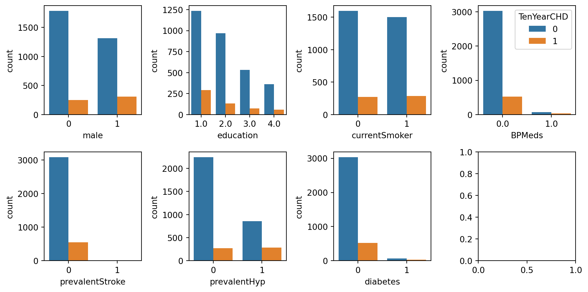
for va in qual_var[:-1]:
tab = pd.crosstab(data_cleaned[va], data_cleaned['TenYearCHD'])
chi2_stat, p_value, dof, expected = chi2_independence_test(tab)
tab_result = pd.concat([tab_result,
pd.DataFrame({
'Chi2-stat': chi2_stat,
'df': dof,
'p-value': p_value}, index=[va])], axis=0)
tab_result.index = qual_var[:-1]
tab_result