Advanced Machine Learning
Code:
AMSI61AML
Course Criteria
Criteria |
Percentage |
|---|---|
| Attendance | 10% |
| Participation & quiz | 10% |
| Midterm Exam or/and Project | 15%+15% |
| Final Exam | 20% |
| Final Project & Presentation | 30% |
Course webpage
Introduction
What’s Machine Learning (ML)?
- Machine = Computer
- Learning = Improving in some task w.r.t some measurement.
“The field of study that gives computers the ability to learn (from data) without being explicitly programmed.”
“A computer program is said to learn from experience \(E\) with respect to some class of tasks \(T\) and performance measure \(P\) if its performance at tasks in \(T\), as measured by \(P\), improves with experience \(E\).”
Why does it matter?
Why does it matter?
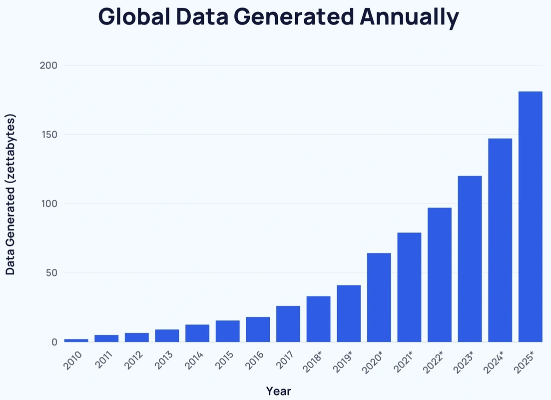
MLis a powerful tool in this era.
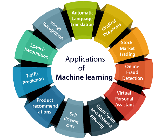
Source: https://www.javatpoint.com/applications-of-machine-learning
Course Outline
Week |
Topic |
|---|---|
| 1 | Naive Bayesian Classifier, LDA & QDA |
| 2 | Logistic Regression & Regularization |
| 3 | KNN & Decision Trees |
| 4 | Ensemble Learning |
| 5 | Model Selection |
| 6 | Hard Clustering |
| 7 | Probabilistic Clustering |
| 8 | Midterm Exam |
| 9 | Dimensional Reduction: PCA, SVD |
| 10 | Association Rules |
| 11 | Markov Decision Process & Q-learning |
| 12 | Upper Confident Bound (PCB) & Thomson sampling |
| 13 | Deep Learning |
| 14 | MLOps |
| 15-16 | ML for SDG & Future Trends |
| 17-18 | Final exam & Projects |
What we will focus on
- Data comprehension:
- What should we focus on when analyzing the data?
- How can data comprehension guide us to the best model?
- Method comprehension:
- How ML models work?
- What models seem to be suitable for a given dataset?
- Pros & cons?
- Practical tasks:
- Quizzes
- Practical labs (TP)
- Projects + presentations…
1. Naive Bayesian Classifier (NBC)
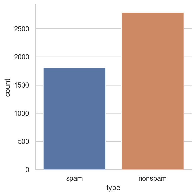
Example: Email spam filter ✉️
- Input \(\text{x}_i=(x_{i1},x_{i2},\dots, x_{id})\):
Bag of wordsof email \(i\). - Label \(y_i\in\{1,0\}\) where \(1=\)
Spam& \(0=\)Nonspam. - Objective: Classify if an email is a spam based on its input.
| make | address | all | num3d | our | over | remove | internet | order | ... | charSemicolon | charRoundbracket | charSquarebracket | charExclamation | charDollar | charHash | capitalAve | capitalLong | capitalTotal | type | ||
|---|---|---|---|---|---|---|---|---|---|---|---|---|---|---|---|---|---|---|---|---|---|
| 3588 | 0.0 | 0.0 | 0.00 | 0.0 | 0.0 | 0.0 | 0.0 | 0.0 | 0.0 | 0.00 | ... | 0.000 | 0.000 | 0.000 | 0.0 | 0.0 | 0.0 | 1.000 | 1 | 5 | nonspam |
| 3192 | 0.0 | 0.0 | 0.17 | 0.0 | 0.0 | 0.0 | 0.0 | 0.0 | 0.0 | 0.17 | ... | 0.267 | 0.802 | 0.118 | 0.0 | 0.0 | 0.0 | 4.808 | 20 | 601 | nonspam |
2 rows × 58 columns
Example: Email spam filter ✉️
- Consider \(3\) inputs:
make,address&capitalTotal. - Suitable graphic\(^{\text{📚}}\): histogram, density, boxplot, violinplot…
import matplotlib.pyplot as plt
_, ax = plt.subplots(1, 3, figsize = (12, 3.5))
sns.histplot(data=spam, x="make", ax=ax[0], binwidth=0.2, hue = "type")
ax[0].set_title("Distribution of 'make'")
sns.histplot(data=spam, x="address", ax=ax[1], binwidth=0.5, hue = "type")
ax[1].set_title("Distribution of 'address'")
sns.histplot(data=spam, x="capitalTotal", ax=ax[2], binwidth=700, hue = "type")
ax[2].set_title("Distribution of 'capitalTotal'")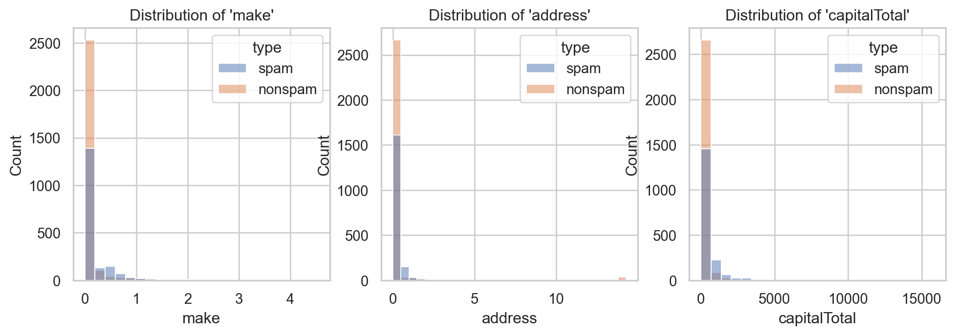
⚠️ Values are too concentrated around \(0\)!
- Use
logscale: too wide range, too dense around \(0\)…
_, ax = plt.subplots(1, 3, figsize = (12, 3.5))
sns.histplot(data=spam, x="make", ax=ax[0], binwidth=0.2, hue = "type")
ax[0].set_title("Distribution of 'make'")
ax[0].set_yscale("log")
sns.histplot(data=spam, x="address", ax=ax[1], binwidth=0.5, hue = "type")
ax[1].set_title("Distribution of 'address'")
ax[1].set_yscale("log")
sns.histplot(data=spam, x="capitalTotal", ax=ax[2], binwidth=700, hue = "type")
ax[2].set_title("Distribution of 'capitalTotal'")
ax[2].set_yscale("log")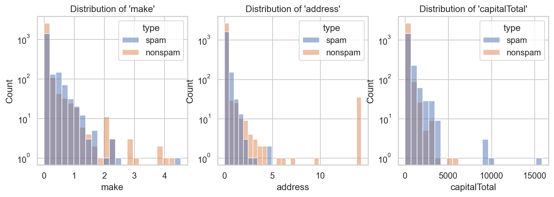
✅ Better, isn’t it?
Example: Email spam filter ✉️
- Consider \(X=(\)
make,address,capitalTotal\()\in\mathbb{R}^3\).
Code
from scipy.stats import gaussian_kde
import numpy as np
x1 = [1.5, 4.2, 5050]
x2 = [1.5, 4.2, 9000]

# Given Y = 1
ker_make = gaussian_kde(spam.make[spam.type=="spam"])
ker_address = gaussian_kde(spam.address[spam.type=="spam"])
ker_capital = gaussian_kde(spam.capitalTotal[spam.type=="spam"])
den11 = [ker_make(x1[0]), ker_address(x1[1]), ker_capital(x1[2])]
den12 = [ker_make(x2[0]), ker_address(x2[1]), ker_capital(x2[2])]
n_spam = np.sum(spam.type=="spam")
n_non = spam.shape[0] - n_spam
pro11 = n_spam/spam.shape[0] * np.prod(den11)
pro12 = n_spam/spam.shape[0] * np.prod(den12)

# Given Y = 0
ker_make = gaussian_kde(spam.make[spam.type=="nonspam"])
ker_address = gaussian_kde(spam.address[spam.type=="nonspam"])
ker_capital = gaussian_kde(spam.capitalTotal[spam.type=="nonspam"])
den01 = [ker_make(x1[0]), ker_address(x1[1]), ker_capital(x1[2])]
den02 = [ker_make(x2[0]), ker_address(x2[1]), ker_capital(x2[2])]
pro01 = n_non/spam.shape[0] * np.prod(den01)
pro02 = n_non/spam.shape[0] * np.prod(den02)

pro01, pro11 = pro01/(pro01+pro11), pro11/(pro01+pro11)
pro02, pro12 = pro02/(pro02+pro12), pro12/(pro02+pro12)
ax[0].vlines([x1[0]], ymin=[0], ymax=[3000], color='black', linestyle = "dashed")
ax[1].vlines([x1[1]], ymin=[0], ymax=[3000], color='black', linestyle = "dashed")
ax[2].vlines([x1[2], x2[2]], ymin=[0], ymax=[3000], color=['red', 'blue'], linestyle = "dashed")
display(fig)
- Type of \(\text{x}_1=(1.5, 4.2, \color{red}{5050})\) and \(\text{x}_2=(1.5, 4.2, \color{blue}{9000})\)?
Recall: Bayes’s Theorem
Bayes’s Theorem
For any two events \(E,H\) with \(\mathbb{P}(E)>0,\) one has \[\begin{equation}\overbrace{\mathbb{P}(H|E)}^{\text{Posterior}}=\frac{\overbrace{\mathbb{P}(E|H)}^{\text{Likelihood}}\times\overbrace{\mathbb{P}(H)}^{\text{Prior}}}{\underbrace{\mathbb{P}(E)}_{\text{Marginal}}}.\end{equation}\]
- \(\mathbb{P}(H)\): Prior belief of having hypothesis \(H\).
- \(\mathbb{P}(E|H)\): If \(H\) is true, how likely for \(E\) to be observed?
- \(\mathbb{P}(H|E)\): If \(E\) is observed, how likely for \(H\) to be true?
- \(\mathbb{P}(E)\): How likely for \(E\) to be observed in general?
Back to email spam filter problem
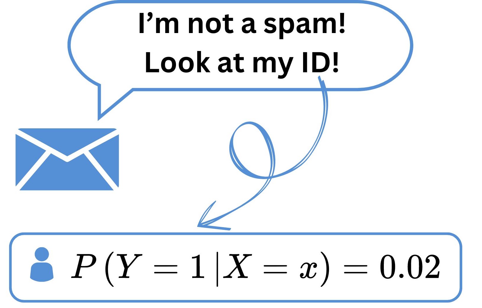
For any email \(\text{x}=(x_1,\dots, x_d)\): \[\mathbb{P}(Y=1|X=\text{x})=\frac{\mathbb{P}^{\small\text{📚}}(X=\text{x}|Y=1)\times\mathbb{P}(Y=1)}{\mathbb{P}(X=\text{x})}.\]
\(\mathbb{P}(Y=1|X=\text{x})^{\small\text{📚}}\) allows us to classify email \(x\): \[\text{Email x} \text{ is a }\begin{cases}\text{spam}& \mbox{if }\mathbb{P}(Y=1|X=\text{x})\geq\delta\\ \text{nonspam}& \mbox{if }\mathbb{P}(Y=1|X=\text{x})<\delta\end{cases}\] for some \(\delta\in (0,1)\). A common choice is \(\delta=0.5\).
Main assumption of NBC
Key quantities in classification
\[\mathbb{P}(Y=1|X=\text{x})\propto \color{red}{\mathbb{P}(X=\text{x}|Y=1)}\times\color{green}{\mathbb{P}(Y=1)}.\]
\(\color{green}{\mathbb{P}(Y=1)}\) can be estimated by \(\frac{n(\text{spams})}{n(\text{emails})}\) ✅
\(\color{red}{\mathbb{P}(X=\text{x}|Y=1)}\) is more complicated (key to different models) ⚠️
Main Assumption of Naive Bayes
Within any class \(k\in\{1,0\}\), the components of \(X|Y=k\) are indpendent i.e., \[\color{red}{\mathbb{P}(X=\text{x}|Y=k)}=\prod_{j=1}^d\mathbb{P}(X_j=x_j|Y=k).\]
Key quantities of NBC
Key quantities in Naive Bayes
\[\mathbb{P}(Y=1|X=\text{x})\propto \color{green}{\mathbb{P}(Y=1)}\color{red}{\prod_{j=1}^d\mathbb{P}(X_j=x_j|Y=1)},\]
- \(\mathbb{P}(X_j=x_j|Y=1)\) can be estimated (in 1D)\(^{\small\text{📚}}\) as follows:
| Type of \(X_j\) | Distribution | Graphic |
|---|---|---|
| Qualitative | Bernoulli, Multinomial… | barplot, countplot |
| Quantitative | Gausian, Exponential… | displot, hist, density… |
Back to email spam filter problem
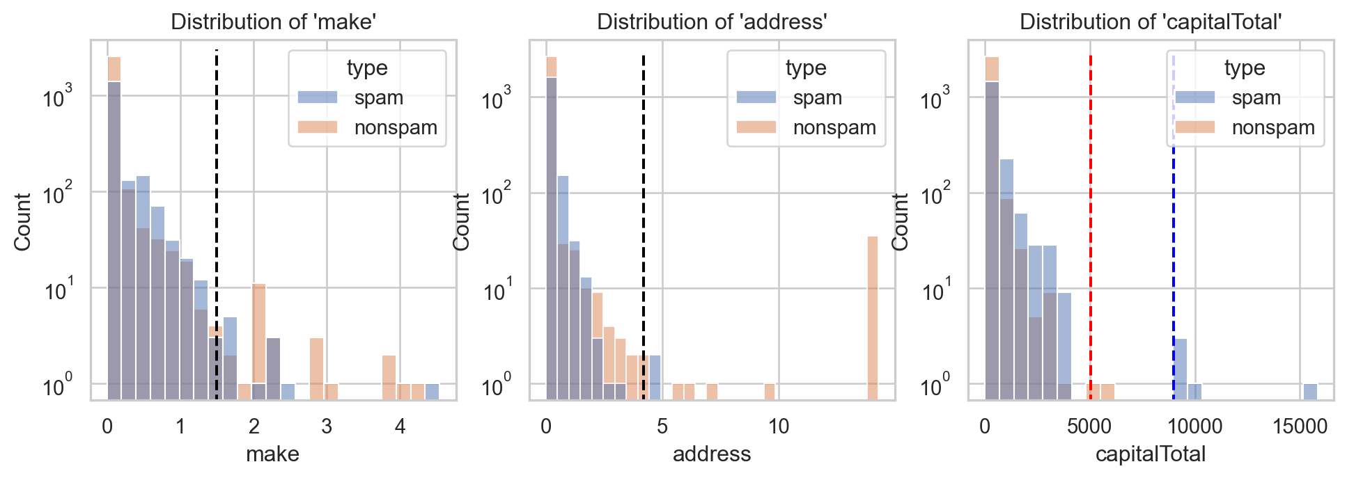
- For \(\text{x}_1=(1.5, 4.2, \color{red}{5050})\) and \(\text{x}_2=(1.5, 4.2, \color{blue}{9000})\):
- \(\mathbb{P}(Y=1|X=\text{x}_1)=\) 3.84e-05.
- \(\mathbb{P}(Y=1|X=\text{x}_2)=\) 1.0, with \(\mathbb{P}(Y=1)=\) 0.394.
\(M\)-class Naive Bayes Classifier
- For any \(d\)-dimensional input \(\text{x}\) and \(k\in\{1,2,...,M\}\):
Key quantity
\[\mathbb{P}(Y=k|X=\text{x})\propto\mathbb{P}(Y=k)\prod_{j=1}^d\mathbb{P}(X_j=x_j|Y=k).\]
Classification rule
\[x\text{ belongs to class }k^*\text{ if }\mathbb{P}(Y=k^*|X=x)=\max_{1\leq k\leq M}\mathbb{P}(Y=k|X=\text{x}).\]
Pros & Cons of NBC
Pros
- Efficiency & simplicity
- Less training data requirement
- Scalability: works well on large and high-dimensional data
- Ability to handle categorical data
- Ability to handle missing data
- Sometimes, it still works well even thought the assumption of
independenceis violeted.
Cons
- May perform poorly when features are highly correlated due to the violation of
independenceassumption. - May not work well for complex relationship.
- Zero probability: when some categories are not presented in some training features.
- Continuous features often be modeled using Gaussian distribution, which might not always be appropriate.
Results on Spam dataset
- Data: \((\text{x},y)\in\mathbb{R}^{57}\times\{0,1\}\).
- Test data: \(20\%\) of total 4601 observations.
from sklearn.naive_bayes import GaussianNB
from sklearn.metrics import confusion_matrix, ConfusionMatrixDisplay
from sklearn.model_selection import train_test_split
sns.set(style="white")
X_train1, X_test1, y_train1, y_test1 = train_test_split(spam.iloc[:,:57], spam.iloc[:,57], test_size = 0.2, random_state=42)
nb1 = GaussianNB()
nb1 = nb1.fit(X_train1, y_train1)
pred1 = nb1.predict(X_test1)
conf1 = confusion_matrix(pred1, y_test1)
con_fig1 = ConfusionMatrixDisplay(conf1)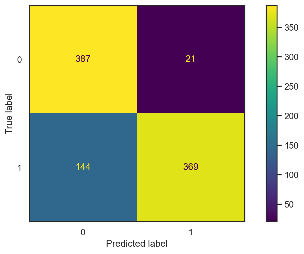
- Accuracy: \[\frac{387+369}{387+369+21+144}\approx 0.821.\]
- Misclassification error: \[1-\text{accuracy}\approx 0.179.\]
- This depends on the split ⚠️
- Input: \(x=(\)
make,address,capitalTotal\()\in\mathbb{R}^3\). - Test data: the same \(20\%\).
X_train2, X_test2, y_train2, y_test2 = train_test_split(spam[["make","address", "capitalTotal"]], spam.iloc[:,57], test_size = 0.2, random_state=42)
nb2 = GaussianNB()
nb2 = nb1.fit(X_train2, y_train2)
pred2 = nb2.predict(X_test2)
conf2 = confusion_matrix(pred2, y_test2)
con_fig2 = ConfusionMatrixDisplay(conf2)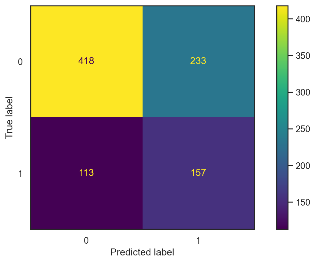
- Accuracy: \[\frac{418+157}{418+157+233+113}\approx 0.624.\]
- Misclassification error: \[1-\text{accuracy}\approx0.376.\]
- This depends on the split ⚠️
Imbalanced data ⚠️
- If the data contains \(95\%\)
nonspam, always guessingnonspamgives \(0.95\) accuracy! Accuracyisn’t the right metric forimbalanceddata ⚠️
Confustion Matrix
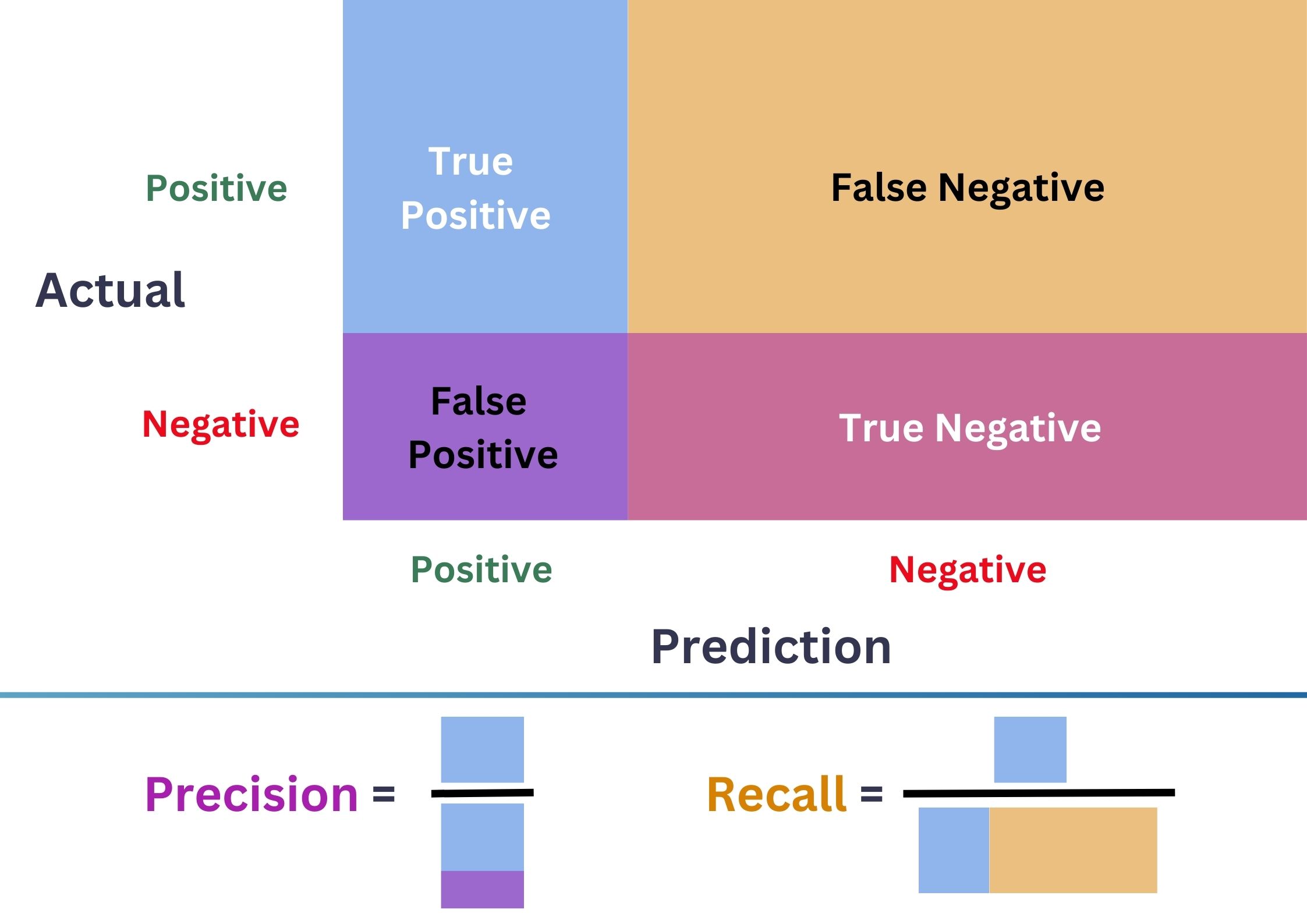
- \(\color{purple}{\text{Precision}}=\frac{\color{CornflowerBlue}{\text{TP}}}{\color{CornflowerBlue}{\text{TP}}+\color{purple}{\text{FP}}}\)
- \(\color{Tan}{\text{Recall}}=\frac{\color{CornflowerBlue}{\text{TP}}}{\color{CornflowerBlue}{\text{TP}}+\color{Tan}{\text{FN}}}\)
- \(\color{ForestGreen}{\text{F1-score}}=\frac{2.\color{purple}{\text{Precision}}.\color{Tan}{\text{Recall}}}{\color{purple}{\text{Precision}}+\color{Tan}{\text{Recall}}}\).
- \(\color{ForestGreen}{\text{F1-score}}\) balances \(\color{purple}{\text{FP}}\) & \(\color{Tan}{\text{FN}}\).
Imbalanced data ⚠️

- \(\color{purple}{\text{Precision}}=\frac{\color{CornflowerBlue}{\text{TP}}}{\color{CornflowerBlue}{\text{TP}}+\color{purple}{\text{FP}}}\)
- \(\color{Tan}{\text{Recall}}=\frac{\color{CornflowerBlue}{\text{TP}}}{\color{CornflowerBlue}{\text{TP}}+\color{Tan}{\text{FN}}}\)
- \(\color{ForestGreen}{\text{F1-score}}=\frac{2.\color{purple}{\text{Precision}}.\color{Tan}{\text{Recall}}}{\color{purple}{\text{Precision}}+\color{Tan}{\text{Recall}}}\).
Code
import plotly.graph_objects as go
x = np.linspace(0,1,20)
y = np.linspace(0,1,20)
z1 = [[2*x[i]*y[j]/(x[i]+y[j]) for j in range(len(y))] for i in range(len(x))]
z2 = [[(x[i]+y[j])/2 for j in range(len(y))] for i in range(len(x))]

camera = dict(
    eye=dict(x=1.7, y=-1.2, z=1.2)
)

fig = go.Figure(go.Surface(x = x,
                           y = y,
                           z = z1,
                           name = "F1-score",
                           colorscale = "Blues",
                           showscale = False))
fig.add_trace(go.Surface(x = x,
                         y = y,
                         z = z2,
                        name = "Mean",
                        colorscale = "Electric",
                        showscale = False))
fig.update_layout(scene = dict(
                    xaxis_title='Precision',
                    yaxis_title='Recall',
                    zaxis_title='Scores'),
                  title = dict(text="F1-score vs Mean",
                               y=0.9,
                               x=0.5,
                               font=dict(size = 30,
                                         color = "#1C66B5")
                              ),
                  scene_camera=camera,
                  width = 560,
                  height = 500)
fig.show()
Imbalanced data ⚠️
Receiver Operating Characteristic Curve (ROC)
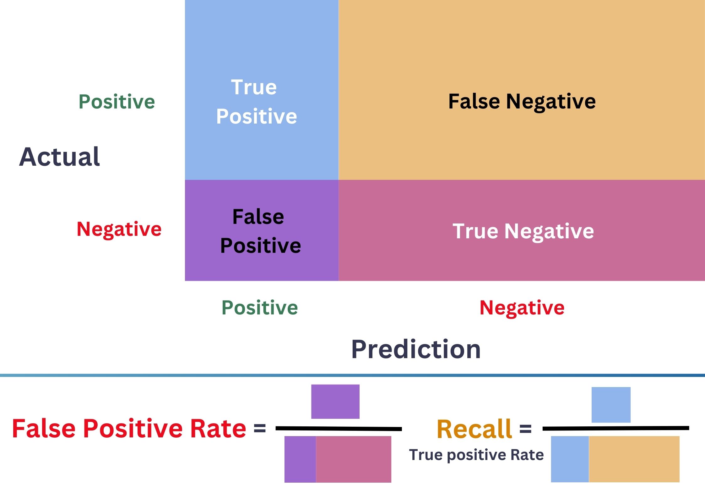
\(\bullet\) ROC \(=\{(\)FPR\(_{\delta}\),TPR\(_{\delta}):\delta\in[0,1]\}\).
\(\bullet\) Better model = Larger Area Under the Curve (AUC).
Code
from plot_metric.functions import BinaryClassification
from plotly.tools import mpl_to_plotly
# Visualisation with plot_metric
y1 = 1*(y_test1 == "spam")
bc1 = BinaryClassification(y1, pr1, labels=["nonspam", "spam"], seaborn_style="whitegrid")

bc2 = BinaryClassification(y1, pr2, labels=["nonspam", "spam"], seaborn_style="whitegrid")

# Figures
a = bc1.plot_roc_curve()
fig_full = plt.gcf()
pl_full = mpl_to_plotly(fig_full)
pl_full.update_layout(width=500, height=450,
                      title=dict(text="ROC Curve of Full model",
                                 font=dict(size=25)),
                      xaxis_title = dict(font=dict(size=20, color = "red")),
                      yaxis_title = dict(text='True Positive Rate (Recall)', font=dict(size=20, color = "#EBB31D")),
                      template='plotly_white')
pl_full.show()
Imbalanced data ⚠️
Receiver Operating Characteristic Curve (ROC)

\(\bullet\) ROC \(=\{(\)FPR\(_{\delta}\),TPR\(_{\delta}):\delta\in[0,1]\}\).
\(\bullet\) Better model = Larger Area Under the Curve (AUC).
Code
bc2 = BinaryClassification(y1, pr2, labels=["nonspam", "spam"], seaborn_style="whitegrid")

# Figures
b = bc2.plot_roc_curve()
fig_3 = plt.gcf()
pl_3 = mpl_to_plotly(fig_3)
pl_3.update_layout(width=500, height=450,
                      title=dict(text="ROC Curve of 3-input model",
                                 font=dict(size=25)),
                      xaxis_title = dict(font=dict(size=20, color = "red")),
                      yaxis_title = dict(text='True Positive Rate (Recall)', font=dict(size=20, color = "#EBB31D")),
                      template='plotly_white')
pl_3.show()
Imbalanced data ⚠️ (Summary)
Confusion matrix
- Precision: controlls FP.
- Recall: controlls FN.
- F1-score: ballances the two.

ROC Curve & AUC
- ROC Curve: ballances TPR and FPR.
- Can be used to select \(\delta\in [0,1]\).
- Better model = Larger AUC.

Imbalanced data ⚠️ (to explore)
- Sampling methods:
- Oversampling: random, SMOTE, SMOTE SVM, ADASYN…
- Undersampling: random, new miss, CNN, Tomek Links…
- Weight adjustment methods (nonparametric)
- Tree-based algorithms, \(k\)-NN, kernel methods…
- Tuning threshold \(\delta\).
- Work with packages that handle imbalanced data:
- Helpful links: Geeks for Geeks, Angelleon Collado, Machine Learning Mastery…
Quiz time 🤗

Showtime 🫣
Quiz time (again) 🤗

Showtime (once more) 🫣
2. Linear, Quadratic & Regularized Discriminant Analysis (LDA, QDA & RDA)
Univariate Gaussian Distribution
Code
import numpy as np
from plotly.subplots import make_subplots
import plotly.graph_objs as go

# define means and covaraince matrix
mu1, Sigma1 = 0, 3

# Simulate points
x1 = np.random.normal(mu1, Sigma1, 100)

# Plot points
fig = go.Figure(go.Scatter(x=x1,
                           y=[0 for i in range(len(x1))],
               mode = "markers",
               name = "Points/Observations",
               showlegend = True,
               marker = dict(size = 6)))
# Density
def density_gaussian1d(x, mu, sigma):
  return 1/((2*np.pi*sigma ** 2) ** (1/2)) * np.exp(-1/2 * (x-mu) ** 2/ sigma ** 2)

x = np.linspace(-10, 10, 50)
y1 = np.array([density_gaussian1d(xi, mu1, Sigma1) for xi in x])

fig.add_trace(
    go.Line(x=x,
            y =y1,
            name = "Density/Possibility",
            showlegend = True))

fig.update_layout(title = dict(text="1D Gaussian Random Variables",
                               x = 0.5,
                               y = 0.98,
                               font=dict(size = 20,
                                          color = "#1C66B5")),
                  width = 450,
                  height = 430,
                  yaxis_title=dict(text='Density'),
                  legend=dict(
                  yanchor="top",
                  y=0.95,
                  xanchor="left",
x=0.01))- Simulate \(x_1,\dots,x_{100}\) with \[x_i\sim{\cal N}(0,3^3).\]
- Desity function: \[f_X(x)=\frac{1}{\sqrt{2\pi\sigma^2}}e^{-\frac{1}{2\sigma^2}(x-\mu)^2},\]
- \(\mathbb{E}(X)=\mu\in\mathbb{R}\)
- \(\mathbb{V}(X)=\mathbb{E}[(X-\mu)^2]=\sigma^2\).
Multivariate Gaussian Distribution
Code
import numpy as np
from plotly.subplots import make_subplots
import plotly.graph_objs as go

# define means and covaraince matrix
mu1, Sigma1 = [0, 0], [[1, 0.5], [0.5, 3]]

# Simulate points
x1 = np.random.multivariate_normal(mean=mu1, cov=Sigma1, size=100)

# Plot points
fig = go.Figure(go.Scatter3d(x=x1[:,0],
                           y=x1[:,1],
                           z=[0 for i in range(x1.shape[0])],
               mode = "markers",
               name = "Points/Observations",
               showlegend = True,
               marker = dict(size = 4)))

# Simulate points
# Density
def density_gaussian2d(x, mu, Sigma):
  return 1/((2*np.pi) ** (len(x)/2) * np.sqrt(np.linalg.det(Sigma))) * np.exp(-1/2 * np.dot(np.dot(x-mu, np.linalg.inv(Sigma)), x-mu))

x = np.linspace(-5, 5, 50)
y = np.linspace(-5, 5, 50)
f1 = np.array([[density_gaussian2d(np.array([xi,yi]), mu1, Sigma1) for xi in x] for yi in y])

fig.add_trace(
    go.Surface(x=x,
               y=y,
               z=f1,
               name = "Density/Possibility",
               opacity=0.3,
               showlegend = True,
               showscale=False))

fig.update_layout(title = dict(text="2D Gaussian Random Variables",
                               x = 0.5,
                               y = 0.98,
                               font=dict(size = 20,
                                          color = "#1C66B5")),
                  width = 400,
                  height = 430,
                  legend=dict(
                  yanchor="top",
                  xanchor="center",
                  y = 0.9,
                  x = 0.5
                ))
fig.update_scenes(zaxis_title_text='Density')- Simulate \(x_1,\dots,x_{100}\) with \(x_i\sim{\cal N}_2\left(\begin{pmatrix} 0 \\ 0 \end{pmatrix}, \begin{pmatrix} 1 & 0.5 \\ 0.5 & 3 \end{pmatrix}\right)\)
- \(d\)-dimensional density: \(f_X(\text{x})=\frac{e^{-\frac{1}{2}(\text{x}-\mu)^t\Sigma^{-1}(\text{x}-\mu)}}{\sqrt{(2\pi)^d|\Sigma|}}.\)
- \(\mathbb{E}(X)=\mu\in\mathbb{R}^d\)
- \(\mathbb{V}(X)=\mathbb{E}[(X-\mu)(X-\mu)^t]=\Sigma\).
Why Gaussian Distribution?
Code
# define means and covaraince matrix
mu1, Sigma1 = [0, 0], [[1, 0], [0, 3]]

mu2, Sigma2  = [5, 5], [[3, -1], [-1, 3]]

mu3, Sigma3 = [-2, 6], [[3, 1.5], [1.5, 1]]

mu4, Sigma4 = [6, 0], [[3, 0.1], [0.1, 0.25]]

x1 = np.random.multivariate_normal(mean=mu1, cov=Sigma1, size=300)
x2 = np.random.multivariate_normal(mean=mu2, cov=Sigma2, size=300)
x3 = np.random.multivariate_normal(mean=mu3, cov=Sigma3, size=300)
x4 = np.random.multivariate_normal(mean=mu4, cov=Sigma4, size=300)

# Save data for later
df_qda = pd.DataFrame({
    "x1" : np.concatenate([x1[:,0], x2[:,0], x3[:,0], x4[:,0]]),
    "x2" : np.concatenate([x1[:,1], x2[:,1], x3[:,1], x4[:,1]]),
    "y" : np.repeat([1,2,3,4], 300)
})

# Plot points
fig0 = go.Figure(go.Scatter3d(x=x1[:,0],
               y = x1[:,1],
               z = [0] * len(x1[:,0]),
               mode = "markers",
               name = "Case 1",
               showlegend = True,
               marker = dict(size = 3)))

fig0.add_trace(
    go.Scatter3d(x=x2[:,0],
               y = x2[:,1],
               z = [0] * len(x1[:,0]),
               mode = "markers",
               name = "Case 2",
               showlegend = True,
               marker = dict(size = 3)))
fig0.add_trace(
    go.Scatter3d(x=x3[:,0],
               y = x3[:,1],
               z = [0] * len(x1[:,0]),
               mode = "markers",
               name = "Case 3",
               showlegend = True,
               marker = dict(size = 3)))
fig0.add_trace(
    go.Scatter3d(x=x4[:,0],
               y = x4[:,1],
               z = [0] * len(x1[:,0]),
               mode = "markers",
               name = "Case 4",
               showlegend = True,
               marker = dict(size = 3)))

# Density
def density_gaussian2d(x, mu, Sigma):
  return 1/((2*np.pi) ** (len(x)/2) * np.sqrt(np.linalg.det(Sigma))) * np.exp(-1/2 * np.dot(np.dot(x-mu, np.linalg.inv(Sigma)), x-mu))

x = np.linspace(-10, 15, 50)
y = np.linspace(-5, 12, 50)
f1 = np.array([[density_gaussian2d(np.array([xi,yi]), mu1, Sigma1) for xi in x] for yi in y])
f2 = np.array([[density_gaussian2d(np.array([xi,yi]), mu2, Sigma2) for xi in x] for yi in y])
f3 = np.array([[density_gaussian2d(np.array([xi,yi]), mu3, Sigma3) for xi in x] for yi in y])
f4 = np.array([[density_gaussian2d(np.array([xi,yi]), mu4, Sigma4) for xi in x] for yi in y])

fig0.add_trace(
    go.Surface(x = x,
               y = y,
               z = f1,
               name = "Density 1",
               showlegend = True,
               opacity=0.5,
               showscale=False))
fig0.add_trace(
    go.Surface(x=x,
               y =y,
               z=f2,
               name = "Density 2",
               opacity=0.5,
               showlegend = True,
               showscale=False))
fig0.add_trace(
    go.Surface(x=x,
               y =y,
               z=f3,
               name = "Density 3",
               opacity=0.5,
               showlegend = True,
               showscale=False))
fig0.add_trace(
    go.Surface(x=x,
               y =y,
               z=f4,
               name = "Density 4",
               showlegend = True,
               opacity=0.5,
               showscale=False))
camera = dict(
    eye=dict(x=0, y=-1.2, z=1.5)
)
fig0.update_layout(title = dict(text="Gaussian models",
                               x = 0.4,
                               y = 0.9,
                               font=dict(size = 20,
                                          color = "#1C66B5")),
                  scene_camera=camera,
                  width = 420,
                  height = 510)
fig0.show()Quadratic Discriminant Analysis
Recall key quantities
\[\mathbb{P}(Y=k|X=\text{x})\propto \color{red}{\mathbb{P}(X=\text{x}|Y=k)}\times\color{green}{\mathbb{P}(Y=k)}.\]
Main Assumption of QDA
For any class \(k\in\{1,\dots,M\}\): \[\color{red}{\mathbb{P}(X=\text{x}|Y=k)}={\cal N}_d(\mu_k,\Sigma_k),\] for some \(\mu_k\in\mathbb{R}^d\) and \(d\times d\)-matrix \(\Sigma\) (to be estimated).
🔑 Within any class, the shape of input \(X\) is assumed to be Gaussian.
Discriminant Function
Goal: Search for class \(k\) such that
\[\begin{align*} \mathbb{P}(Y=k|X=\text{x})=&\arg\max_{1\leq m\leq M}\mathbb{P}(Y=m|X=\text{x})\\ =&\arg\max_{1\leq m\leq M} \mathbb{P}(Y=m)\mathbb{P}(X=\text{x}|Y=m)\\ =&\arg\max_{1\leq m\leq M} \log\left(\mathbb{P}(Y=m)\mathbb{P}(X=\text{x}|Y=m)\right)\\ =&\arg\max_{1\leq m\leq M} \delta_m(\text{x}), \end{align*}\] where \(\delta_m(\text{x})\) measures the association of the input \(\text{x}\) to the class \(k\) and is defined by \[\delta_m(\text{x})=\color{green}{\log(\pi_m)}-\color{blue}{\log(|\Sigma_m|)}-\color{red}{\frac{1}{2}(\text{x}-\mu_m)^t\Sigma_m^{-1}(\text{x}-\mu_m)}\] with \(\pi_m=\mathbb{P}(Y=m), \mu_m\in\mathbb{R}^d\) and matrix \(\Sigma_m\) to be estimated \(\forall m=1,\dots,M\).
Boundary Decision of QDA
Definition: Boundary Decision
Boundary decision of 2 classes \(k\) and \(j\) is the set of inputs \(\text{x}\in\mathbb{R}^d\) satisfying: \[\mathbb{P}(Y=k|X=\text{x})=\mathbb{P}(Y=j|X=\text{x}).\]
Boundary Decision of QDA
- Boundary decision between class \(k\) and \(j\) in QDA are inputs \(\text{x}\) s.t \(\delta_k(\text{x})=\delta_j(\text{x})\).
- It’s a
Quadratic Formof \(\text{x}: \text{x}^tA\text{x}+v^t\text{x}+c=0\), where \(A\) is a \(d\times d\) symmetric matrix, \(v\in\mathbb{R}^d\) and \(c\in\mathbb{R}\) and depend on \(\pi_k,\pi_j,\mu_k,\mu_j,\Sigma_k\) and \(\Sigma_j\). - Such a boundary is more flexible than linear boundary, but easily overfit the data!
Implementation of QDA
Implementation\(^{\text{📚}}\)
- Given: Training data \({\cal D}_n\{(\text{x}_1,y_1),\dots,(\text{x}_n,y_n)\}\) and the query input \(\text{x}\).
for\(k\)in range(M)estimate:- \(\hat{\pi}_k=n_k/n\) where \(n_k=\text{card}(\{i:y_i=k\})\) (estimate prior \(\mathbb{P}(Y=k)\))
- \(\hat{\mu}_k=\frac{1}{n_k}\sum_{i:y_i=k}\text{x}_i\) (estimate mean of class \(k\))
- \(\hat{\Sigma}_k=\frac{1}{n_k}\sum_{i:y_i=k}(\text{x}_i-\hat{\mu}_k)(\text{x}_i-\hat{\mu}_k)^t\) (estimate covariance matrix of class \(k\))
- Compute \(\delta_k(\text{x})=\log(\hat{\pi}_k)-\log(|\hat{\Sigma}_k|)-\frac{1}{2}(\text{x}-\hat{\mu}_k)^t\hat{\Sigma}_k^{-1}(\text{x}-\hat{\mu}_k)\)
return\(k\) with the largest value of \(\delta_k(\text{x})\).
Linear Dicriminant Analysis (LDA)
- QDA can be expensive when \(M\) is large.
- LDA is achieved by imposing the following assumption.
Main Assumption of LDA
In LDA, we assume that the input \(X\) has the same covariance matrix within all classes, i.e., \[\Sigma_k=\Sigma, \forall k=1,\dots,M.\] In other words, \(X\) has the same shape for all classes.
Code
# define means and covaraince matrix
mu1, Sigma1 = [0, 0], [[2, 0], [0, 2]]

mu2, Sigma2  = [5, 5], [[3, 0], [0, 3]]

mu3, Sigma3 = [-2, 6], [[1, 0], [0, 1]]

mu4, Sigma4 = [6, 0], [[1.75, 0], [0, 1.75]]

x1 = np.random.multivariate_normal(mean=mu1, cov=Sigma1, size=300)
x2 = np.random.multivariate_normal(mean=mu2, cov=Sigma2, size=300)
x3 = np.random.multivariate_normal(mean=mu3, cov=Sigma3, size=300)
x4 = np.random.multivariate_normal(mean=mu4, cov=Sigma4, size=300)

# Save data for later
df_lda = pd.DataFrame({
    "x1" : np.concatenate([x1[:,0], x2[:,0], x3[:,0], x4[:,0]]),
    "x2" : np.concatenate([x1[:,1], x2[:,1], x3[:,1], x4[:,1]]),
    "y" : np.repeat([1,2,3,4], 300)
})

# Plot points
fig1 = go.Figure(go.Scatter3d(x=x1[:,0],
               y = x1[:,1],
               z = [0] * len(x1[:,0]),
               mode = "markers",
               name = "Case 1",
               showlegend = True,
               marker = dict(size = 3)))

fig1.add_trace(
    go.Scatter3d(x=x2[:,0],
               y = x2[:,1],
               z = [0] * len(x1[:,0]),
               mode = "markers",
               name = "Case 2",
               showlegend = True,
               marker = dict(size = 3)))
fig1.add_trace(
    go.Scatter3d(x=x3[:,0],
               y = x3[:,1],
               z = [0] * len(x1[:,0]),
               mode = "markers",
               name = "Case 3",
               showlegend = True,
               marker = dict(size = 3)))
fig1.add_trace(
    go.Scatter3d(x=x4[:,0],
               y = x4[:,1],
               z = [0] * len(x1[:,0]),
               mode = "markers",
               name = "Case 4",
               showlegend = True,
               marker = dict(size = 2)))

# Density
def density_gaussian2d(x, mu, Sigma):
  return 1/((2*np.pi) ** (len(x)/2) * np.sqrt(np.linalg.det(Sigma))) * np.exp(-1/2 * np.dot(np.dot(x-mu, np.linalg.inv(Sigma)), x-mu))

x = np.linspace(-5, 10, 50)
y = np.linspace(-5, 10, 50)
f1 = np.array([[density_gaussian2d(np.array([xi,yi]), mu1, Sigma1) for xi in x] for yi in y])
f2 = np.array([[density_gaussian2d(np.array([xi,yi]), mu2, Sigma2) for xi in x] for yi in y])
f3 = np.array([[density_gaussian2d(np.array([xi,yi]), mu3, Sigma3) for xi in x] for yi in y])
f4 = np.array([[density_gaussian2d(np.array([xi,yi]), mu4, Sigma4) for xi in x] for yi in y])

fig1.add_trace(
    go.Surface(x = x,
               y = y,
               z = f1,
               name = "Density 1",
               showlegend = True,
               opacity=0.5,
               showscale=False))
fig1.add_trace(
    go.Surface(x=x,
               y =y,
               z=f2,
               name = "Density 2",
               opacity=0.5,
               showlegend = True,
               showscale=False))
fig1.add_trace(
    go.Surface(x=x,
               y =y,
               z=f3,
               name = "Density 3",
               opacity=0.5,
               showlegend = True,
               showscale=False))
fig1.add_trace(
    go.Surface(x=x,
               y =y,
               z=f4,
               name = "Density 4",
               showlegend = True,
               opacity=0.5,
               showscale=False))
camera = dict(
    eye=dict(x=0, y=-1.2, z=1.5)
)
fig1 = fig1.update_layout(
                   title = dict(text=r'$\Sigma_k\text{ in LDA}$',
                                y=0.9,
                                x=0.25,
                                font=dict(size = 20,
                                          color = "#1C66B5")
                              ),
                  scene_camera=camera,
                  width = 320,
                  height = 250)

import ipywidgets as ipw
fig0.update_layout(title = dict(text=r'$\Sigma_k\text{ in QDA}$',
                                y=0.9,
                                x=0.25,
                                font=dict(size = 20,
                                          color = "#1C66B5")
                              ),
                  scene_camera=camera,
                  width = 320,
                  height = 250)
fig0 = go.FigureWidget(fig0)
fig1 = go.FigureWidget(fig1)
ipw.HBox([fig0, fig1])
LDA is slightly simpler than QDA
Discriminant Function
- In LDA, \(\delta_k(\text{x})=\log(\pi_k)-\frac{1}{2}(\text{x}-\mu_k)^t\Sigma^{-1}(\text{x}-\mu_k).\)
Boundary Decision of LDA
- The boundary decision takes
Linear Formof \(\text{x}\): \[\text{x}^tv+c=0,\] where \(v\in\mathbb{R}^d\) and \(c\in\mathbb{R}\) and depend on \(\pi_k,\pi_j,\mu_k,\mu_j\) and \(\Sigma\).
Code
import matplotlib as mpl
from matplotlib import colors
import matplotlib.pyplot as plt
from sklearn.inspection import DecisionBoundaryDisplay

# Functions for ellipses and boudary decision
def plot_ellipse(mean, cov, color, ax):
    v, w = np.linalg.eigh(cov)
    u = w[0] / np.linalg.norm(w[0])
    angle = np.arctan(u[1] / u[0])
    angle = 180 * angle / np.pi  # convert to degrees
    # filled Gaussian at 2 standard deviation
    ell = mpl.patches.Ellipse(
        mean,
        2 * v[0] ** 0.5,
        2 * v[1] ** 0.5,
        angle=180 + angle,
        facecolor=color,
        edgecolor="black",
        linewidth=2,
    )
    ell.set_clip_box(ax.bbox)
    ell.set_alpha(0.4)
    ax.add_artist(ell)

def plot_result(estimator, X, y, ax):
    cmap = colors.ListedColormap(["tab:red", "tab:blue"])
    DecisionBoundaryDisplay.from_estimator(
        estimator,
        X,
        response_method="predict_proba",
        plot_method="pcolormesh",
        ax=ax,
        cmap="RdBu",
        alpha=0.3,
    )
    DecisionBoundaryDisplay.from_estimator(
        estimator,
        X,
        response_method="predict_proba",
        plot_method="contour",
        ax=ax,
        alpha=1.0,
        levels=[0.5],
    )
    y_pred = estimator.predict(X)
    X_right, y_right = X[y == y_pred], y[y == y_pred]
    X_wrong, y_wrong = X[y != y_pred], y[y != y_pred]
    ax.scatter(X_right[:, 0], X_right[:, 1], c=y_right, s=20, cmap=cmap, alpha=0.5)
    ax.scatter(
        X_wrong[:, 0],
        X_wrong[:, 1],
        c=y_wrong,
        s=30,
        cmap=cmap,
        alpha=0.9,
        marker="x",
    )
    ax.scatter(
        estimator.means_[:, 0],
        estimator.means_[:, 1],
        c="yellow",
        s=200,
        marker="*",
        edgecolor="black",
    )
    if isinstance(estimator, LDA):
        covariance = [estimator.covariance_] * 2
    else:
        covariance = estimator.covariance_
    plot_ellipse(estimator.means_[0], covariance[0], "tab:red", ax)
    plot_ellipse(estimator.means_[1], covariance[1], "tab:blue", ax)

    ax.set_box_aspect(1)
    ax.spines["top"].set_visible(False)
    ax.spines["bottom"].set_visible(False)
    ax.spines["left"].set_visible(False)
    ax.spines["right"].set_visible(False)
    ax.set(xticks=[], yticks=[])

fig, axs = plt.subplots(nrows=1, ncols=2, sharex="row", sharey="row", figsize=(8, 12))

from sklearn.discriminant_analysis import LinearDiscriminantAnalysis as LDA
from sklearn.discriminant_analysis import QuadraticDiscriminantAnalysis as QDA

lda = LDA(solver="svd", store_covariance=True)
qda = QDA(store_covariance=True)

for ax_row, X, y in zip(
    (axs,),
    (df_qda[["x1", "x2"]].to_numpy()[:600,:], ),
    (df_qda['y'].to_numpy()[:600], ),
):
    lda.fit(X, y)
    plot_result(lda, X, y, ax_row[0])
    qda.fit(X, y)
    plot_result(qda, X, y, ax_row[1])

axs[0].set_title("Boundary decision of LDA")
axs[1].set_title("Boundary decision of QDA")
plt.show()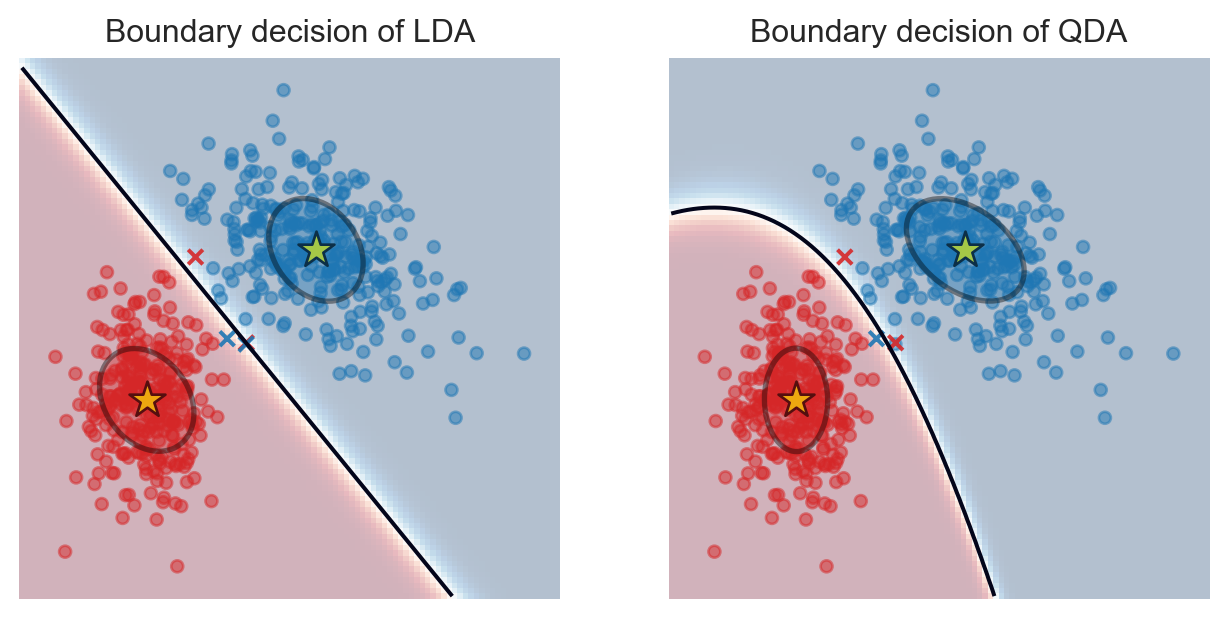
Implementation of LDA
Implementation\(^{\text{📚}}\)
- Given: Training data \({\cal D}_n\{(\text{x}_1,y_1),\dots,(\text{x}_n,y_n)\}\) and the query input \(\text{x}\).
- \(\hat{\Sigma}=\frac{1}{n-M}\sum_{k=1}^M\sum_{i:y_i=k}(\text{x}_i-\hat{\mu}_k)(\text{x}_i-\hat{\mu}_k)^t\) (esimate common covariance matrix)
for\(k\)in range(M)estimate:- \(\hat{\pi}_k=n_k/n\) where \(n_k=\text{card}(\{i:y_i=k\})\) (estimate prior \(\mathbb{P}(Y=k)\))
- \(\hat{\mu}_k=\frac{1}{n_k}\sum_{i:y_i=k}\text{x}_i\) (estimate mean of class \(k\))
- Compute \(\delta_k(\text{x})=\log(\hat{\pi}_k)-\frac{1}{2}(\text{x}-\hat{\mu}_k)^t\hat{\Sigma}^{-1}(\text{x}-\hat{\mu}_k)\)
return\(k\) with the largest value of \(\delta_k(\text{x})\).
Regularized Discriminant Analysis
Regularized DA (RDA) is about regularizing the convariance matrices\(^{\text{📚}}\)
- LDA & QDA can be combined, for example, Friedman (1989) proposed: \[\hat{\Sigma}_k(\alpha)=\alpha\hat{\Sigma}+(1-\alpha)\hat{\Sigma}_k,\] for some \(\alpha\in[0,1]\).
- The common covariance \(\hat{\Sigma}\) can also be shrunk toward the scalar covariance: \[\hat{\Sigma}(\lambda)=\lambda\hat{\Sigma}+(1-\lambda)\hat{\sigma}^2I_d,\] for some \(\lambda\in[0,1]\).
- Define a family of covariance matrices \(\hat{\Sigma}_k(\alpha,\lambda)\) for \((\alpha,\lambda)\in[0,1]^2\) to be tuned.
Regularization effect in action
Code
mu1, Sigma1 = [0, 0], np.array([[1, 0], [0, 3]])

mu2, Sigma2  = [5, 5], np.array([[3, -1], [-1, 3]])

mu3, Sigma3 = [-2, 6], np.array([[3, 1.5], [1.5, 1]])

mu4, Sigma4 = [6, 0], np.array([[3, 0.1], [0.1, 0.25]])


df_alpha = np.row_stack([np.random.multivariate_normal(mean=mu1,
                                                          cov=Sigma1,
                                                          size=100),
                         np.random.multivariate_normal(mean=mu2,
                                                          cov=Sigma2,
                                                          size=100),
                         np.random.multivariate_normal(mean=mu3,
                                                          cov=Sigma3,
                                                          size=100),
                         np.random.multivariate_normal(mean=mu4,
                                                          cov=Sigma4,
                                                          size=100)])

df0 = df_alpha.copy()

Sigma0 = np.array([[1.25, 0], [0, 1.25]])

df_final = np.row_stack([np.random.multivariate_normal(mean=mu1,
                                                          cov=Sigma0,
                                                          size=100),
                         np.random.multivariate_normal(mean=mu2,
                                                          cov=Sigma0,
                                                          size=100),
                         np.random.multivariate_normal(mean=mu3,
                                                          cov=Sigma0,
                                                          size=100),
                         np.random.multivariate_normal(mean=mu4,
                                                          cov=Sigma0,
                                                          size=100)])

alpha_list = np.linspace(0, 1, 15)
alphas = [0] * 400
classes = np.repeat([int(i) for i in range(1,5)], 100)

for alpha in alpha_list[1:]:
  temp = df0 + alpha * (df_final - df0)
  df_alpha = np.row_stack([df_alpha,  temp])
  alphas = np.concatenate((alphas, [alpha] * 400))
  classes = np.concatenate((classes, np.repeat([int(i) for i in range(1,5)], 100)))

df_alpha = np.column_stack([df_alpha, alphas, classes])
df_alpha = pd.DataFrame(df_alpha)
df_alpha.columns = ['x1', 'x2', 'alpha', 'class']
df_alpha['alpha'] = df_alpha['alpha'].round(3)
df_alpha['class'] = df_alpha['class'].astype(int)
df_alpha['class'] = df_alpha['class'].astype(str)

import plotly.graph_objects as go
import matplotlib.pyplot as plt
import plotly.express as px

df_alpha["dummy_size"] = 1
fig = px.scatter(df_alpha, x="x1", y="x2", animation_frame="alpha", color="class", hover_data='class', size="dummy_size", size_max = 10)
fig.update_layout(title = dict(text=r'Transition of covariance',
                                y=1,
                                x=0.2,
                                font=dict(size = 30,
                                          color = "#1C66B5")
                              ),
    width=500, height = 520,
    transition = {'duration': 500})
fig.show()
Right covariances \(\approx\) right shapes!
\(\alpha\in[0,1]\) balances the trade-off between the covariance \(\Sigma_k\) (QDA) and the common variance \(\Sigma\) (LDA): \[\Sigma_k(\alpha)=\alpha\Sigma+(1-\alpha)\Sigma_k.\]
In practice, \(\alpha\) is tuned using
cross-validationtechnique (later).
Summary of LDA, QDA & RDA
- Main assumption:
Normalityof inputs within each class: \[\mathbb{P}(X=x|Y=k)={\cal N}(\mu_k,\Sigma_k)\] - Assumptions on covariance matrices lead to different methods:
- QDA: \(\hat{\Sigma}_k\) are computed differently.
- LDA: \(\hat{\Sigma}_k=\hat{\Sigma}\) are all the same.
- RDA: \(\hat{\Sigma}_k(\alpha,\lambda)=(1-\alpha)\hat{\Sigma}_k+\alpha[\lambda\hat{\Sigma}+(1-\lambda)\hat{\sigma}^2I_d]\).
- No method is always the best, it depends on the data.
LDA, QDA & RDA on Spam dataset
- Same \(20\%\) test data of total 4601 observations.
sns.set(style="white")
# Build LDA object & predict
lda = LDA(solver="svd", store_covariance=True)
lda1 = lda.fit(X_train1, y_train1)
pred1_lda = lda1.predict(X_test1)
conf1_lda = confusion_matrix(pred1_lda, y_test1)
con_fig1_lda = ConfusionMatrixDisplay(conf1_lda)

qda = QDA(store_covariance=True)
qda1 = qda.fit(X_train1, y_train1)
pred1_qda = qda1.predict(X_test1)
conf1_qda = confusion_matrix(pred1_qda, y_test1)
con_fig1_qda = ConfusionMatrixDisplay(conf1_qda)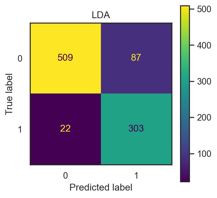
- LDA accuracy: 0.882.
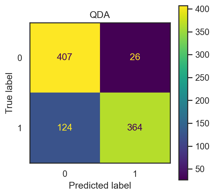
- QDA accuracy: 0.882.
- Input: \(x=(\)
make,address,capitalTotal\()\in\mathbb{R}^3\).
lda = LDA(solver="svd", store_covariance=True)
lda2 = lda.fit(X_train2, y_train2)
pred2_lda = lda2.predict(X_test2)
conf2_lda = confusion_matrix(pred2_lda, y_test2)
con_fig2_lda = ConfusionMatrixDisplay(conf2_lda)

qda = QDA(store_covariance=True)
qda2 = qda.fit(X_train2, y_train2)
pred2_qda = qda2.predict(X_test2)
conf2_qda = confusion_matrix(pred2_qda, y_test2)
con_fig2_qda = ConfusionMatrixDisplay(conf2_qda)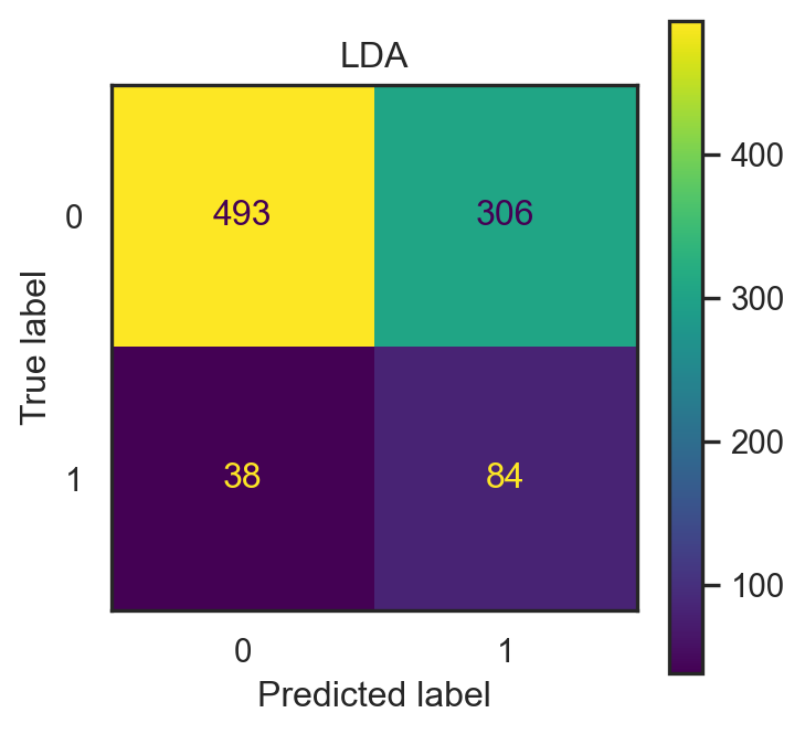
- LDA accuracy: 0.626.
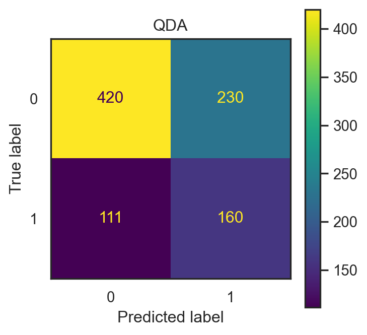
- QDA accuracy: 0.626.
Coming in the TP 😁!
Pros & Cons
Pros
- Effective for multiclass problems (compute & compare \(\delta_k(x),\forall k\).)
- Computationally efficient (LDA).
- Allow to compute class probabilities.
- Minimal hyperparameter tuning.
- Stability with small sample sizes (LDA but not QDA).
Cons
- Assumption of multivariate normality may not be suitable.
- Sensitivity to outliers.
- Less flexible with non-linear boundaries (especially for LDA).
- Require enough data in each class for variance estimates (QDA & RDA)…
Quiz time 🤗

Showtime 🫣
🥳 It’s party time 🥂
📋 View party menu here: Party 1 Menu.
🫠 Download party invitation here: Party 1 Invitation Letter.


