🗺️ Content
Motivation & Tools
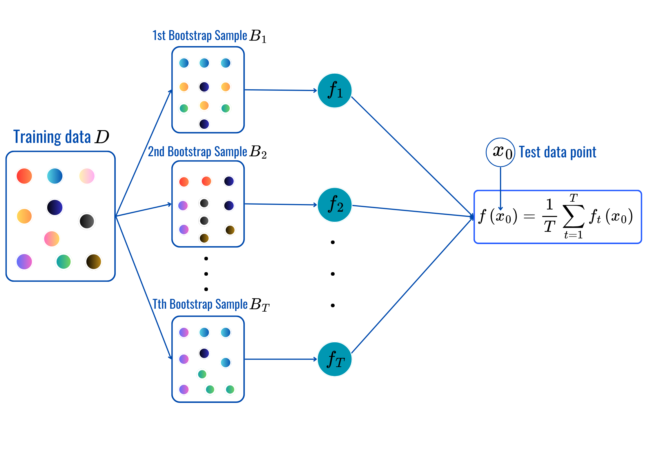
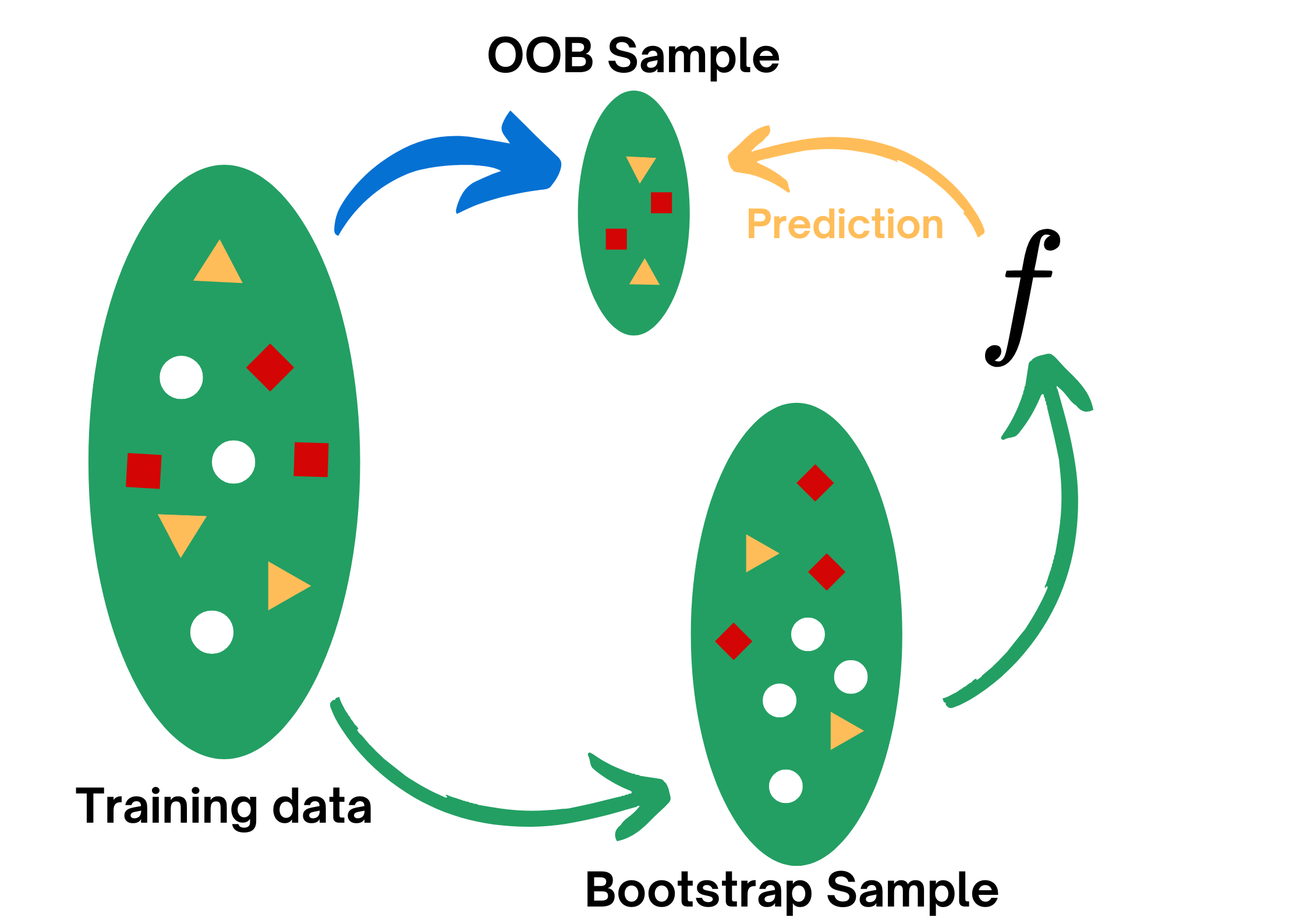
Bagging: Random Forest
Boosting: Adaboost, XGBoost…
Concensual aggregation: COBRA, KernelCOBRA, MixCOBRA
Stacking: SuperLearner

![]()
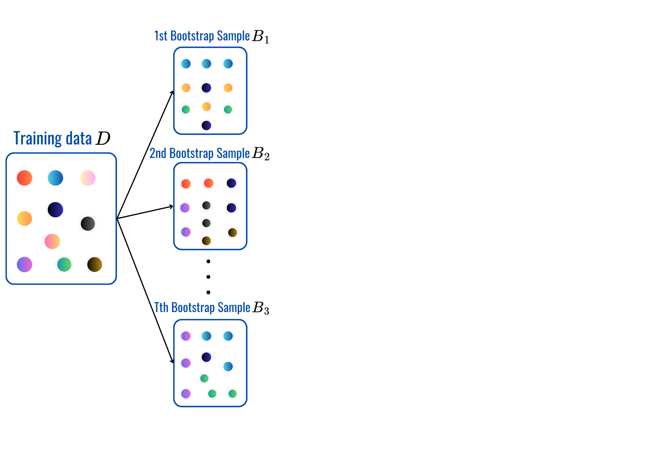
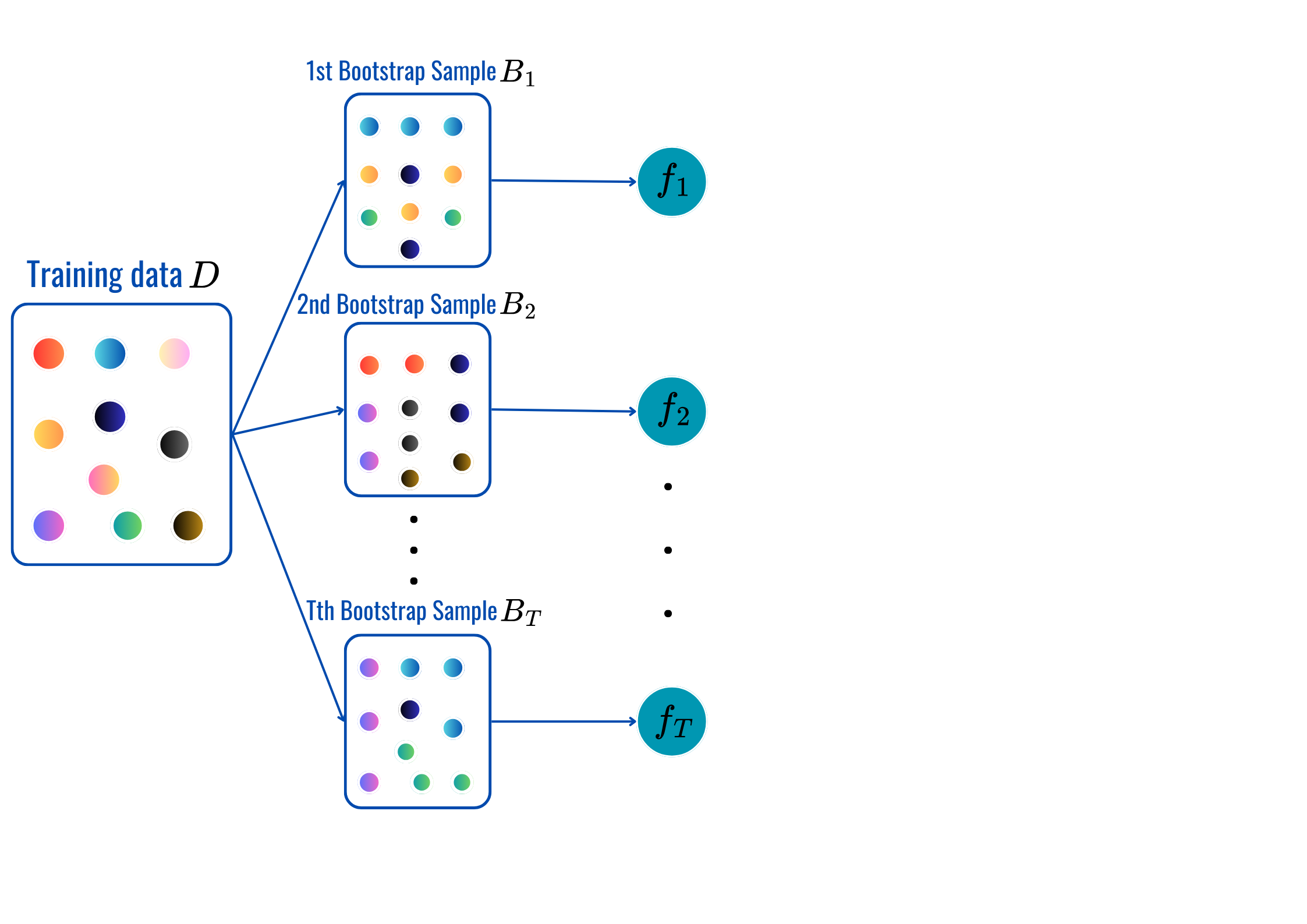
for t = 1,2,...,T:
Prediction: (same as before).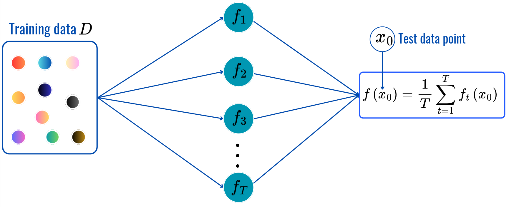


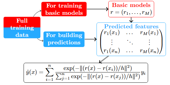
\[\varphi(h)=\frac{1}{K}\sum_{k=1}^K\sum_{(\text{x}_i,y_i)\in F_j}(\hat{y}_i-y_i)^2.\]

\[\varphi(\alpha,\beta)=\frac{1}{K}\sum_{k=1}^K\sum_{(\text{x}_i,y_i)\in F_j}(\hat{y}_i-y_i)^2.\]
![]()
