Advanced Machine Learning

     

Lecturer: Dr. HAS Sothea

Code: AMSI61AML

🧊 Dimensional Reduction Techniques

🗺️ Content

• Motivation
  

• Principal Component Analysis (PCA)
  

• t-distribution Stochastic Neighbor Embeding (t-SNE)
  

• Autoencoder
  

Motivation

Why reducing dimension?

• High-dimensional data means “large number of columns/fat data”.

• There are many problems when dealing with high-dimensional data:
  • Curse of dimensionality
  • Noise
  • Complexity: analysis and computation
  • Cannot be visualized
  • Prone to overfitting…
• The core idea of “Dimensional Reduction” is

High-dimensional data often live in smaller dimensional spaces.

Principal Component Analysis (PCA)

Setting

• Given data matrix: \(X\in\mathbb{R}^{n\times d}\),

	X	Y	Z
0	-0.959	-0.808	-1.409
1	-2.439	0.870	-1.008
2	0.661	0.043	1.787
3	-3.891	-1.206	-4.043
4	0.618	1.229	0.470
5	1.310	0.082	0.454
6	0.822	-2.479	-1.142
7	4.057	1.629	6.200
8	1.932	1.685	4.132

• PCA is a process of representing \(X\) in a new coordinate system (basis) such that:
  • Each column has maximum variation along its direction.
  • All columns are perpendicular/independent.

Principal Component Analysis (PCA)

First Principal Direction \(\color{blue}{\vec{u}_1}\)

• PCA is a process of representing \(X\) in a new coordinate system such that:
  • Each column has maximum variation along its direction.
  • All columns are perpendicular/independent.

Objective of PCA

• Without loss of generality, assume \(X\) is centered: \(\overline{X}_j=0,\forall j=1,\dots,d\).
• Objective: Finding \(\color{blue}{U}\in\mathbb{R}^{d\times d}\) such that \[\tilde{X}=X\color{blue}{U}\text{ s.t: }\begin{cases}\|\tilde{X}_j\|^2\text{ is maximized}\\\tilde{X}_j\perp\tilde{X}_k,\forall j\neq k.\end{cases}\]

• The objective of PCA can be reduced to finding each column of \(\color{blue}{U}\in\mathbb{R}^{d}\).

First Principal Direction \(\color{blue}{\vec{u}_1}\)

• We define the 1st principal direction \(\color{blue}{\vec{u}_1}\in\mathbb{R}^{d}\): \[\begin{align*}\color{blue}{\vec{u}_1}&=\arg\max_{\vec{w}\in\mathbb{R}^d:\|\vec{w}\|=1}\|X\vec{w}\|^2\\ &=\arg\max_{\vec{w}\in\mathbb{R}^d:\|\vec{w}\|=1}\vec{w}^TX^TX\vec{w}.\end{align*}\]

• This problem can be solved using Lagragian Method 👇

📚 Hertzman et al. (2015)
📚 Appendix E. of Bishop et al. (2006).

Principal Component Analysis (PCA)

Lagragian Method for \(\color{blue}{\vec{u}_1}\)

• Problem: Find \(\color{blue}{\vec{u}_1}\in\mathbb{R}^d\) such that

\[\begin{align*}\color{blue}{\vec{u}_1}&=\arg\max_{\vec{w}\in\mathbb{R}^d:\|\vec{w}\|=1}\vec{w}^TX^TX\vec{w}.\end{align*}\]

• Lagragian at \(\color{red}{\vec{w}}\in\mathbb{R}^d\) and \(\color{red}{\lambda}\in\mathbb{R}\),

\[\begin{align*} {\cal L}(\color{red}{\vec{w}},\color{red}{\lambda})&=f(\color{red}{\vec{w}})+\color{red}{\lambda} g(\color{red}{\vec{w}})\\ &=\color{red}{\vec{w}}^TX^TX\color{red}{\vec{w}}+\color{red}{\lambda}(1-\|\color{red}{\vec{w}}\|^2)\\ &=\color{red}{\vec{w}}^TX^TX\color{red}{\vec{w}}+\color{red}{\lambda}(1-\color{red}{\vec{w}}^T\color{red}{\vec{w}}). \end{align*}\]

• The solution may be obtained by setting the derivatives (gradients) of \(\cal L\) to 0 i.e., \(\nabla {\cal L}=0\).

• Verify that the solution \(\color{blue}{\vec{u}_1}\in\mathbb{R}^d\) and \(\color{blue}{\lambda}\in\mathbb{R}\) of the system \[\begin{cases}\frac{\partial {\cal L}(\color{blue}{\vec{u}_1},\color{blue}{\lambda})}{\partial \color{blue}{\vec{u}_1}}=0\\ \frac{\partial {\cal L}(\color{blue}{\vec{u}_1},\color{blue}{\lambda})}{\partial \color{blue}{\lambda}}=0\end{cases},\] satisfies \(X^TX\color{blue}{\vec{u}_1}=\color{blue}{\lambda\vec{u}_1}.\)
• This implies that the 1st principal direction \(\color{blue}{\vec{u}_1}\) is the eigenvector of \(X^TX\) corresponding to the eigenvalue \(\color{blue}{\lambda}\).

Principal Component Analysis (PCA)

\(k\)-th principal direction \(\color{blue}{\vec{u}_k}, k\geq 2\)

\(k\)-th Principal direction \(\color{blue}{\vec{u}_k}\)

• For any \(k\in\{2,\dots,d\}\), let \[\color{red}{\widehat{X}_k}=X-\sum_{j=1}^{k-1}X\color{blue}{\vec{u}_j\color{blue}{\vec{u}_j^T}},\] then the \(k\)-th Principal direction \(\color{blue}{\vec{u}_k}\) is the unit vector, orthogonal to \(\{\color{blue}{\vec{u}_j}:1\leq j\leq k-1\}\), and the variation of projected data on its direction is maximized: \[\begin{align*}\color{blue}{\vec{u}_k}&=\arg\max_{\vec{w}\in\mathbb{R}^d:\|\vec{w}\|=1}\vec{w}^T\color{red}{\widehat{X}_k^T\widehat{X}_k}\vec{w}.\end{align*}\]

• Proof: Using Lagragian multiplier just like the case of \(\color{blue}{\vec{u}_1}\).

Solution to PCA problem

• Solution to our original problem is \[\color{blue}{U}=[\color{blue}{\vec{u}_1}| \color{blue}{\vec{u}_2| \dots | \color{blue}{\vec{u}_d}}]\in\mathbb{R}^d.\] where \(\color{blue}{\vec{u}_j}\) is the \(j\)-th eigenvector of \(X^TX\) corresponding to eigenvalue \(\color{blue}{\lambda_j}>0\).
• The rotated data is defined by: \[\color{blue}{\tilde{X}}=X\color{blue}{U}.\]
• The variation along each direction \[\sum_{j=1}^d\|X_j\|^2=\sum_{j=1}^d\|\color{blue}{\tilde{X}_j}\|^2=\sum_{j=1}^d\color{blue}{\lambda_j^2}\]

Principal Component Analysis (PCA)

Implementing PCA

Unnormalized PCA

• Given data: \(X\in\mathbb{R}^{n\times d}\)
• Centering \(X_c=\underbrace{X}_{n\times d} -\underbrace{\mathbb{1}_n}_{n\times n}\underbrace{X}_{n\times d}/n.\)
• Perform Eigenvalue Decomposition on covariance matrix \(V=X_c^TX_c\): \[V=\color{blue}{U}\Sigma \color{blue}{U}^T,\]
  • \(\color{blue}{U}\): matrix of eigenvectors
  • \(\Sigma=\text{diag}(\lambda_1,\dots,\lambda_d)\): diagonal matrix of eigenvalues \(\lambda_1\geq \dots\geq \lambda_d\geq 0\).

Normalized PCA

• Given data: \(X\in\mathbb{R}^{n\times d}\)
• Standardizing: compute std matrix \(D=\text{diag}(\widehat{\sigma}_1,\dots,\widehat{\sigma}_d)\) and standardized data \(Z=(\underbrace{X}_{n\times d} -\underbrace{\mathbb{1}_n}_{n\times n}\underbrace{X}_{n\times d}/n)D^{-1}.\)
• Perform Eigenvalue Decomposition on correlation matrix \(C=Z^TZ/(n-1)\): \[C=\color{blue}{U}\Sigma \color{blue}{U}^T.\]
• Rotated data: \(\color{blue}{\tilde{X}}=X\color{blue}{U}.\) [👉 Demo]

Principal Component Analysis (PCA)

Dimensional reduction/Reconstruction

Dimensional Reduction

• Reduction to \(k\) dimensions (\(k<d\)) is done by \(\tilde{X}_k=\tilde{X}[:,:k].\)
• Quality of representation on each direction: \(\left[\frac{\lambda_1}{\sum_{j=1}^d\lambda_j},\dots,\frac{\lambda_k}{\sum_{j=1}^d\lambda_j}\right].\)
• Variation explained by \(k\) dimensions: \(\frac{\sum_{j=1}^k\lambda_j}{\sum_{j=1}^d\lambda_j}\times 100.\)
• For visualization, one can choose \(k=2\) or \(3\). [👉 Demo]

* Total variation of X: 15.25

	X	Y	Z
0	-0.959	-0.808	-1.409
1	-2.439	0.870	-1.008
2	0.661	0.043	1.787
3	-3.891	-1.206	-4.043
4	0.618	1.229	0.470

* Total variation of projection: 15.2

	PC1	PC2	PC3
0	-2.424	-0.173	-0.197
1	-2.287	2.086	-0.406
2	1.239	-0.292	-0.558
3	-6.119	1.163	-0.709
4	0.509	0.555	0.818

Principal Component Analysis (PCA)

Dimensional reduction/Reconstruction

Dimensional Reduction

• Reduction to \(k\) dimensions (\(k<d\)) is done by \(\tilde{X}_k=\tilde{X}[:,:k].\)
• Quality of representation on each direction: \(\left[\frac{\lambda_1}{\sum_{j=1}^d\lambda_j},\dots,\frac{\lambda_k}{\sum_{j=1}^d\lambda_j}\right].\)
• Variation explained by \(k\) dimensions: \(\frac{\sum_{j=1}^k\lambda_j}{\sum_{j=1}^d\lambda_j}\times 100.\)
• For visualization, one can choose \(k=2\) or \(3\). [👉 Demo]

Reconstruction

• The reconsution is defined by: \[\color{red}{X_k^{\text{rec}}}=\tilde{X}_k\color{blue}{U[:,:k]^T}.\]

• Best low-rank approximation shows that this reconstruction \(\color{red}{X_k^{\text{rec}}}\) is the best \(k\)-rank approximation of \(X\) with respect to Frobenius norm, i.e., \[\color{red}{X_k^{\text{rec}}}=\arg\min_{M_k:r(M_k)\leq k}\|X-M_k\|_F,\] where \(\|.\|_F\) is the Frobenius norm.

Principal Component Analysis (PCA)

Summary

• PCA captures and arranges directions with largest, 2nd largest,… variation into the 1st, 2nd, … column using Spectral Theorem (Eigenvalue decomposition).
• These directions are contained in the eigenvector matrix of Covariance (unnormalized) or Correlation matrix (normalized) of the data.
• The variation along each direction is given by the corresponding eigenvalues: \(\lambda_1>\dots>\lambda_d\).
• Our goal is to explore dimensional reduction and reconstruction power of PCA, however, it can be used in Data Analysis, EDA, Data Summary…
• Remark: Many highly correlated columns indicates effective dimensional reduction (the first two PCs can capture significant variation).

\(t\)-distribution Stochastic Neighbor Embedding (\(t\)-SNE)

Setting

• Suppose \(X\in\mathbb{R}^{n\times d}\) with large \(d\).

Objective

\(t\)-SNE aims at finding lower dimensional (LD) representation of \(X\) (2 or 3) so that the distribution among LD data is similar to the original data.

• Hinton and Roweis (2002) proposed Stochastic Embedding Neighbor (SNE) and \(t\)-SNE is its improved version [see Laurens, \(t\)-SNE Page].

from sklearn.manifold import TSNE

# Prepare the t-SNE model
tsne = TSNE(n_components=2, random_state=42)

# Fit and transform the data
X_tsne = tsne.fit_transform(X[:1000,:])  # Use a subset for faster computation
df_tsne = pd.DataFrame(X_tsne, columns=['Component 1', 'Component 2'])
df_tsne['label'] = y_train[:1000]
fig_tsne = px.scatter(df_tsne, x="Component 1", y="Component 2", color="label")
fig_tsne.update_layout(height=420, width=500, title="t-SNE visualization on MNIST")
fig_tsne.show()

\(t\)-distribution Stochastic Neighbor Embedding (\(t\)-SNE)

Original and embedding distribution in \(t\)-SNE

• Gaussian similarity probability between original points \(\text{x}_i,\text{x}_j\in\mathbb{R}^d\): \[p_{i,j}=\frac{e^{-\|\text{x}_i-\text{x}_j\|^2/(2\sigma^2)}}{\sum_{k\neq \ell:k,\ell=1}^n e^{-\|\text{x}_k-\text{x}_{\ell}\|^2/(2\sigma^2)}}.\]

• \(t\)-distribution probability between embedded data points \(\text{z}_i,\text{z}_j\in\mathbb{R}^{d'} (d'<d)\): \[q_{i,j}=\frac{(1+\|\text{z}_i-\text{z}_j\|^2)^{-1}}{\sum_{k\neq \ell:k,\ell=1}^n (1+\|\text{z}_k-\text{z}_{\ell}\|^2)^{-1}}.\]

\(t\)-SNE

Optimization for LD data \(z_i\)

• In the first proposed method (SNE in Hinton and Roweis (2002)), \(q_{i,j}\) was also Gaussian similarity. This often leads to Crowding Problem.
• Q1: How do we find LD data \(z_i\)?
• We can measure the proximity between vector (or matrix) of similarity probabilities on HD data \(P=(p_{i,j})\) and on LD data \(Q=(q_{i,j})\) using Kullback-Leibler divergence: \[D_{KL}(P||Q)=\sum_{i,j}p_{i,j}\log\left(\frac{p_{i,j}}{q_{i,j}}\right).\]

• Gradient of KL w.r.t \(z_i\):

\[\frac{\partial KL}{\partial z_i}=4\sum_{j}(p_{i,j}-q_{i,j})(z_i-z_j)(1+\|z_i-z_j\|^2)^{-1}.\]

Gradient Descent With Momentum

• Data: \(X=\{\text{x}_1,\dots,\text{x}_n\}\).
• Perplexity: Perp (effective local neighbors between 5 and 50).
• Parameters: max_iter, learning rate: \(\eta\), momentum \(\alpha(t)\).
• Result: LD data \(Z=\{z_1,\dots,z_n\}\).
• Begin:
  • Compute \(p_{i,j}\)
  • Initialize: \(Z^{(0)}=\{z_1^{(0)},\dots,z_n^{(0)}\}\)
  • for t=1 to max_iter do:
    • Compute \(q_{i,j}\) and gradient: \(\frac{\partial KL}{\partial z_i}\)
    • Update: \(Z^{(t)}=Z^{(t-1)}+\eta\frac{\partial KL}{\partial z_i}+\alpha(t)(Z^{(t-1)}-Z^{(t-2)})\).
• End. [👉 Demo]

\(t\)-SNE

Summary

• \(t\)-SNE is a dimentional reduction technique aiming at searching for neighbors of points in a lower-dimensional space (2 or 3) especially for visualization.
• High-dimensional data \(X\) is converted to pairwise similarity probability \(P=(p_{i,j})\) according to how close they are.
• The pairwise similarity probability \(Q=(q_{i,j})\) of low-dimensional data points is defined based on \(t\)-distribution of degree 1 or Cauchy distribution.
• The proximity between \(P\) and \(Q\) is measured using KL divergence.
• The LD data \(z_i\) are estimated by minimizing KL divergence using Gradient Descent with Momontum.

Johnson-Lindenstrauss Lemma (JL)

Setting

• Given data points: \(X\in\mathbb{R}^{n\times d}\)
• JL lemma: result allows us to project data \(\text{x}_i,\text{x}_j\in\mathbb{R}^d\) onto a smaller subspace \(\widehat{\text{x}}_i, \widehat{\text{x}}_j\in\mathbb{R}^{d'}\) with \(d'<d\) such that the Euclidean distance is nearly preserved with high probability, i.e., for any \(\varepsilon>0\): \[\mathbb{P}_{\widehat{\text{x}}_i,\widehat{\text{x}}_j}\left(\left|\frac{\|\widehat{\text{x}}_i-\widehat{\text{x}}_j\|_{d'}^2}{\|\text{x}_i-\text{x}_j\|_d^2}-1\right|>\varepsilon\right)\approx 0.\]

Johnson-Lindenstrauss Lemma (JL)

Lemma

Johnson-Lindenstrauss Lemma (Gaussian matrix projection)

Let \(X=\{\text{x}_1,\dots,\text{x}_n\}\subset\mathbb{R}^d\) be \(n\) points in \(d\)-dimensional Euclidean space \(\mathbb{R}^d\), and let \({\cal G}=(G_{i,j})\) with \(G_{k,j}\overset{iid}{\sim}{\cal N}(0,1/d')\) for \(k=1,\dots,d\) and \(j=1,\dots,\color{blue}{d'}\) with \(\color{blue}{d'}<d\). Let also \(\widehat{\text{x}}_i={\cal G}\text{x}_i\) and \(\widehat{\text{x}}_j={\cal G}\text{x}_j\) be two points of \(\mathbb{R}^{d'}\), thus for any \(\varepsilon\in (0,1)\) one has \[\mathbb{P}_{\cal G}\left(\left|\frac{\|\widehat{\text{x}}_i-\widehat{\text{x}}_j\|_{\color{blue}{d'}}^2}{\|\text{x}_i-\text{x}_j\|_d^2}-1,\forall i,j\right|> \varepsilon\right)< 2ne^{-\color{blue}{d'}(\varepsilon^2/2-\varepsilon^3/3)}.\]

• Proof: see for example: Kevin (2016) or Has (2022).

Johnson-Lindenstrauss Lemma (JL)

When should we consider JL?

• JL lemma focuses on preserving pair of Euclidean distances between data points when projecting.
• It’s suitable for problem involving measuring Euclidean distances between high-dimensional data points: \(k\)-NN, KMeans clustering, Kernel smoothing methods… [👉 Demo]

AutoEncoders

Introduction

• Autoencoders are a type of DNN used for learning efficient codings of input data.
• It’s an unsupervised learning method that works by compressing data into a lower-dimensional representation (encoding) and then reconstructing it back to its original form (decoding).

AutoEncoders

Main components / Loss

• Data: \(X\in\mathbb{R}^{n\times d}\).
• Encoder: \(E:\mathbb{R}^d\to\mathbb{R}^{d'}\) encodes original data into lower-dimensional representation called Latent Representation.
• Decoder: \(D:\mathbb{R}^{d'}\to\mathbb{R}^{d}\) reconstructs back the original data from their Latent Representation.

Loss

• Training optimal \(\color{blue}{E^*}\) and \(\color{blue}{D^*}\) networks can be simply formulated as: \[(\color{blue}{E^*},\color{blue}{D^*})=\arg\min_{E,D} \frac{1}{n}\sum_{i=1}^n\ell(\text{x}_i,D[E(\text{x}_i)]).\]

• This is equivalent to training two neural networks at once.

• AE is in fact a generalization of PCA, while PCA finds the optimal linear subs-space (hyperplane) for the projected data, AE is able to learn non-linear manifold embedding [see Elad Plaut (2018)].

AutoEncoders

Other types

• Sparse Autoencoders: \(\color{blue}{E^*}\) and \(\color{blue}{D^*}\) networks are trained with penalization.
  • \(L_1\) regularization for regression: \[(\color{blue}{E^*},\color{blue}{D^*})=\arg\min_{E,D} \frac{1}{n}\sum_{i=1}^n\ell(\text{x}_i,D[E(\text{x}_i)])+\lambda\sum|\color{blue}{W}_{E,D}|.\]
  • KL divergence for classification: \[(\color{blue}{E^*},\color{blue}{D^*})=\arg\min_{E,D} \frac{1}{n}\sum_{i=1}^n\ell(\text{x}_i,D[E(\text{x}_i)])+\lambda\sum_{j}\color{blue}{\text{KL}}(p\|\hat{p}_j).\]

AutoEncoders

Other types

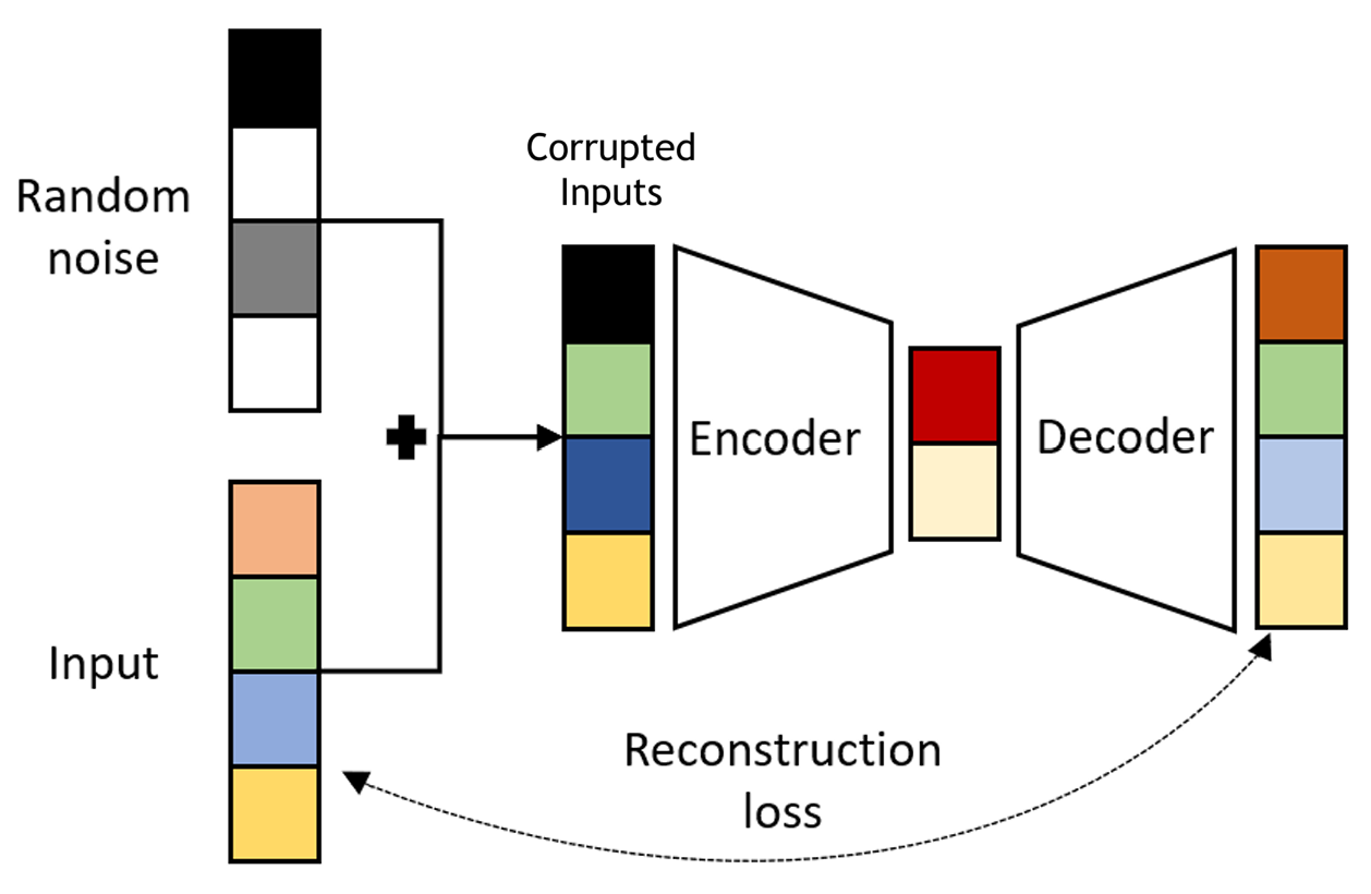
• Denoising Autoencoders: \(\color{blue}{E^*}\) and \(\color{blue}{D^*}\) networks are trained just like before, and the noisy input \(\tilde{\text{x}}_i\) is obtained by, for example, \(\tilde{\text{x}}_i\sim {\cal N}(\text{x}_i,\sigma^2I_d).\)

• Variational Autoencoders (VAE): see for example, Sec. 3 of Bank et al. (2021). [👉 Demo]

🥳 It’s party time 🥂

📋 View party menu here: Party 7 Menu.

🫠 Download party invitation here: Party 7 Invitation Letter.