Abalone dataset
The dataset is available here: https://www.kaggle.com/datasets/rodolfomendes/abalone-dataset.
import kagglehub# Download latest version = kagglehub.dataset_download("rodolfomendes/abalone-dataset" )# Import data import pandas as pd= pd.read_csv(path + "/abalone.csv" )
Warning: Looks like you're using an outdated `kagglehub` version (installed: 0.3.6), please consider upgrading to the latest version (0.3.7).
0
M
0.455
0.365
0.095
0.5140
0.2245
0.1010
0.150
15
1
M
0.350
0.265
0.090
0.2255
0.0995
0.0485
0.070
7
2
F
0.530
0.420
0.135
0.6770
0.2565
0.1415
0.210
9
3
M
0.440
0.365
0.125
0.5160
0.2155
0.1140
0.155
10
4
I
0.330
0.255
0.080
0.2050
0.0895
0.0395
0.055
7
print (f"Number of rows: { data. shape[0 ]} " )print (f"Number of columns: { data. shape[1 ]} " )
Number of rows: 4177
Number of columns: 9
1. EDA
Sex                object
Length            float64
Diameter          float64
Height            float64
Whole weight      float64
Shucked weight    float64
Viscera weight    float64
Shell weight      float64
Rings               int64
dtype: object
count
4177.000000
4177.000000
4177.000000
4177.000000
4177.000000
4177.000000
4177.000000
4177.000000
mean
0.523992
0.407881
0.139516
0.828742
0.359367
0.180594
0.238831
9.933684
std
0.120093
0.099240
0.041827
0.490389
0.221963
0.109614
0.139203
3.224169
min
0.075000
0.055000
0.000000
0.002000
0.001000
0.000500
0.001500
1.000000
25%
0.450000
0.350000
0.115000
0.441500
0.186000
0.093500
0.130000
8.000000
50%
0.545000
0.425000
0.140000
0.799500
0.336000
0.171000
0.234000
9.000000
75%
0.615000
0.480000
0.165000
1.153000
0.502000
0.253000
0.329000
11.000000
max
0.815000
0.650000
1.130000
2.825500
1.488000
0.760000
1.005000
29.000000
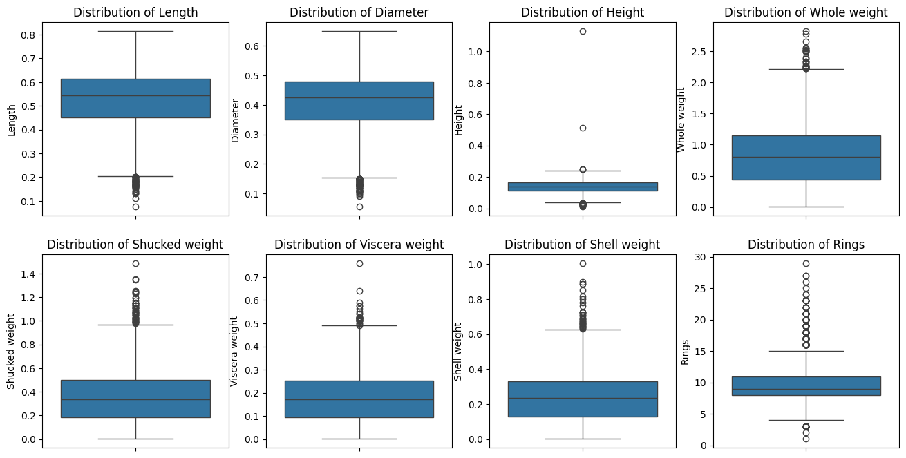
There are missing values (abalone with 0 heights). We shall handle this.
= data.loc[data.Height > 0 ]
count
4175.000000
4175.00000
4175.000000
4175.000000
4175.000000
4175.000000
4175.000000
4175.000000
mean
0.524065
0.40794
0.139583
0.829005
0.359476
0.180653
0.238834
9.935090
std
0.120069
0.09922
0.041725
0.490349
0.221954
0.109605
0.139212
3.224227
min
0.075000
0.05500
0.010000
0.002000
0.001000
0.000500
0.001500
1.000000
25%
0.450000
0.35000
0.115000
0.442250
0.186250
0.093500
0.130000
8.000000
50%
0.545000
0.42500
0.140000
0.800000
0.336000
0.171000
0.234000
9.000000
75%
0.615000
0.48000
0.165000
1.153500
0.502000
0.253000
0.328750
11.000000
max
0.815000
0.65000
1.130000
2.825500
1.488000
0.760000
1.005000
29.000000
print (f'Number of duplicated data: { data. duplicated(). sum ()} ' )
Number of duplicated data: 0
1.1 Univariate Analysis
import seaborn as snsimport matplotlib.pyplot as pltimport plotly.express as px= data.select_dtypes(include= "number" ).columns= plt.subplots(2 ,4 , figsize= (16 , 8 ))for i, va in enumerate (quan_cols):= data, y= va, ax= axs[i// 4 , i % 4 ])// 4 , i % 4 ].set_title(f"Distribution of { va} " )
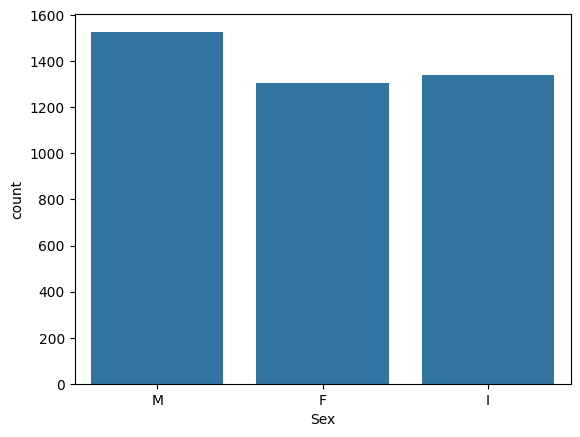
= data, x= "Sex" )
1.2 Bivariate Analysis
= 'number' ).corr()
Length
1.000000
0.986802
0.828108
0.925217
0.897859
0.902960
0.898419
0.556464
Diameter
0.986802
1.000000
0.834298
0.925414
0.893108
0.899672
0.906084
0.574418
Height
0.828108
0.834298
1.000000
0.819886
0.775621
0.798908
0.819596
0.557625
Whole weight
0.925217
0.925414
0.819886
1.000000
0.969389
0.966354
0.955924
0.540151
Shucked weight
0.897859
0.893108
0.775621
0.969389
1.000000
0.931924
0.883129
0.420597
Viscera weight
0.902960
0.899672
0.798908
0.966354
0.931924
1.000000
0.908186
0.503562
Shell weight
0.898419
0.906084
0.819596
0.955924
0.883129
0.908186
1.000000
0.627928
Rings
0.556464
0.574418
0.557625
0.540151
0.420597
0.503562
0.627928
1.000000
= 'number' ).corr(method= "spearman" )
Length
1.000000
0.983299
0.888124
0.972600
0.956790
0.952600
0.948662
0.603954
Diameter
0.983299
1.000000
0.895651
0.971290
0.950422
0.948328
0.954896
0.622487
Height
0.888124
0.895651
1.000000
0.915963
0.874163
0.900535
0.922130
0.657403
Whole weight
0.972600
0.971290
0.915963
1.000000
0.977038
0.975222
0.970197
0.630440
Shucked weight
0.956790
0.950422
0.874163
0.977038
1.000000
0.947581
0.918465
0.538956
Viscera weight
0.952600
0.948328
0.900535
0.975222
0.947581
1.000000
0.938893
0.613930
Shell weight
0.948662
0.954896
0.922130
0.970197
0.918465
0.938893
1.000000
0.692991
Rings
0.603954
0.622487
0.657403
0.630440
0.538956
0.613930
0.692991
1.000000
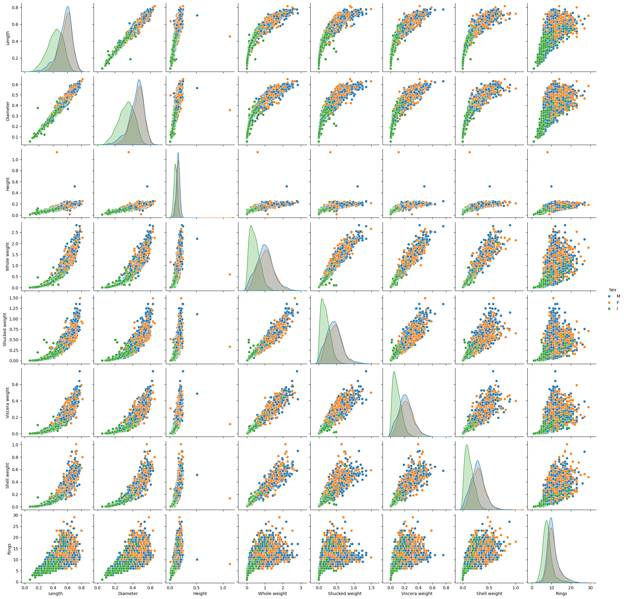
= (16 ,16 ))= data, hue= "Sex" )
<Figure size 1600x1600 with 0 Axes>
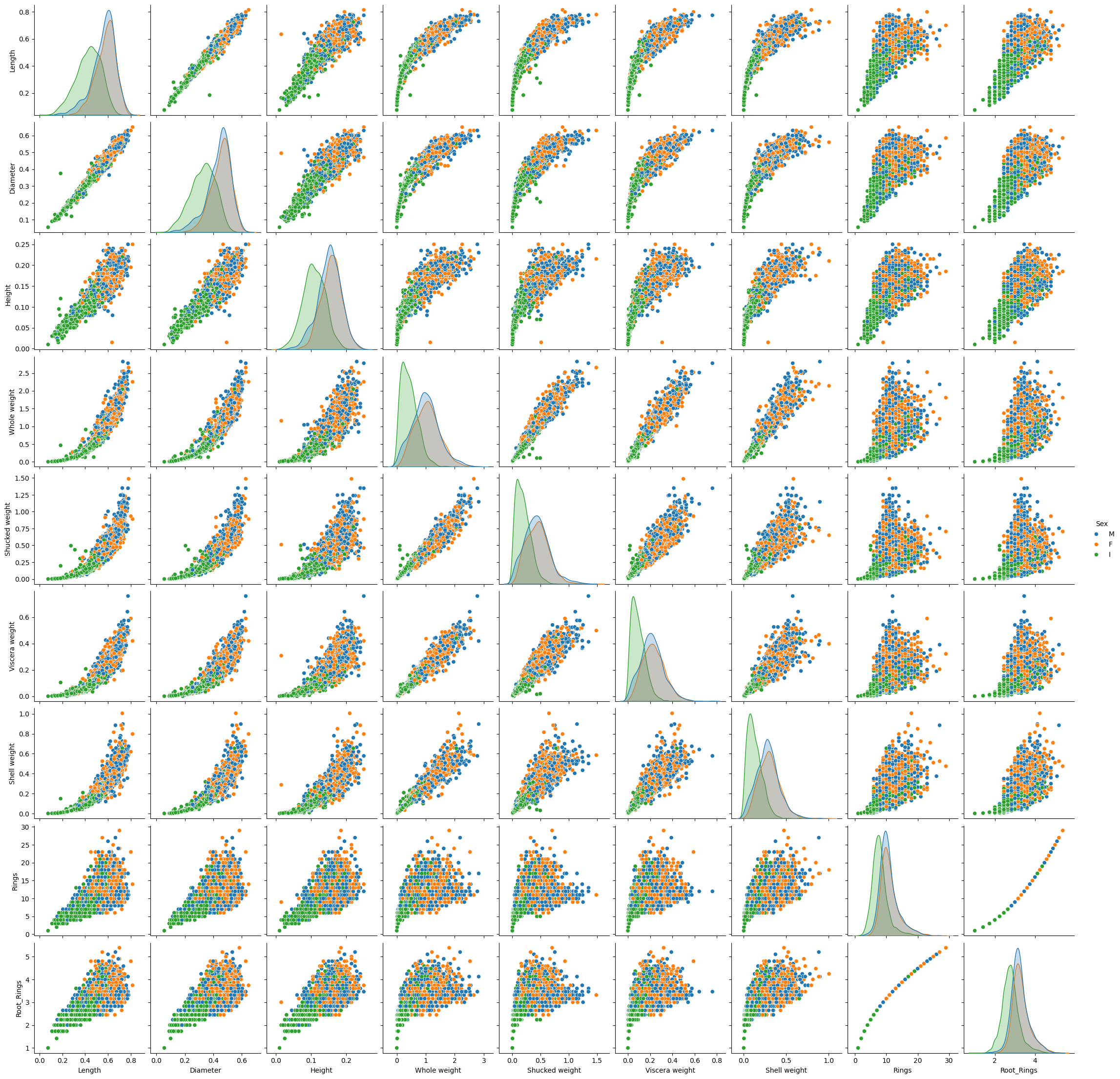
Height has low correlation with the target Rings but this is likely due to the 2 weird data point with large height but small rings. One can remove these data points. Moreover the target spread widely at large values of inputs. One can scale the target to improve the connection.
= dataimport numpy as np'Height' ] > 0.5 ].index, inplace= True )'Root_Rings' ] = data['Rings' ].map (lambda x: np.sqrt(x))= data1, hue= "Sex" )
= ['Sex' ]).corr()
Length
1.000000
0.986794
0.900868
0.925328
0.898129
0.903033
0.898363
0.556572
0.609433
Diameter
0.986794
1.000000
0.907187
0.925499
0.893330
0.899716
0.906026
0.574551
0.626043
Height
0.900868
0.907187
1.000000
0.888850
0.837485
0.866757
0.891857
0.610107
0.651990
Whole weight
0.925328
0.925499
0.888850
1.000000
0.969370
0.966290
0.955954
0.540621
0.574118
Shucked weight
0.898129
0.893330
0.837485
0.969370
1.000000
0.931831
0.883194
0.421156
0.460780
Viscera weight
0.903033
0.899716
0.866757
0.966290
0.931831
1.000000
0.908133
0.503977
0.540612
Shell weight
0.898363
0.906026
0.891857
0.955954
0.883194
0.908133
1.000000
0.628169
0.654175
Rings
0.556572
0.574551
0.610107
0.540621
0.421156
0.503977
0.628169
1.000000
0.991914
Root_Rings
0.609433
0.626043
0.651990
0.574118
0.460780
0.540612
0.654175
0.991914
1.000000
= ['Sex' ]).corr(method= "spearman" )
Length
1.000000
0.983282
0.888776
0.972587
0.956831
0.952555
0.948606
0.603924
0.603924
Diameter
0.983282
1.000000
0.896281
0.971271
0.950446
0.948276
0.954847
0.622477
0.622477
Height
0.888776
0.896281
1.000000
0.916451
0.874402
0.901073
0.922828
0.658139
0.658139
Whole weight
0.972587
0.971271
0.916451
1.000000
0.977044
0.975198
0.970182
0.630489
0.630489
Shucked weight
0.956831
0.950446
0.874402
0.977044
1.000000
0.947578
0.918476
0.539061
0.539061
Viscera weight
0.952555
0.948276
0.901073
0.975198
0.947578
1.000000
0.938835
0.613942
0.613942
Shell weight
0.948606
0.954847
0.922828
0.970182
0.918476
0.938835
1.000000
0.693018
0.693018
Rings
0.603924
0.622477
0.658139
0.630489
0.539061
0.613942
0.693018
1.000000
1.000000
Root_Rings
0.603924
0.622477
0.658139
0.630489
0.539061
0.613942
0.693018
1.000000
1.000000
2. Models
from sklearn.model_selection import train_test_splitfrom sklearn.ensemble import RandomForestRegressor, ExtraTreesRegressorfrom sklearn.metrics import mean_squared_error
2.1 Bagging: Random Forest & Extra-Trees
import numpy as np= pd.get_dummies(data["Sex" ], drop_first= True )= pd.concat([x_cat, data.iloc[:,1 :- 1 ]], axis= 1 )= data['Rings' ].map (lambda x: np.sqrt(x))= train_test_split(X,y, test_size= 0.3 , random_state= 42 )print (X_train.shape, y_train.shape)print (X_test.shape, y_test.shape)
(2921, 10) (2921,)
(1252, 10) (1252,)
= RandomForestRegressor(n_estimators= 300 )= rf.predict(X_test)print (f"RMSE: { np. sqrt(mean_squared_error(y_test, y_pred_rf))} " )
RMSE: 0.004429570403170732
= ExtraTreesRegressor(n_estimators= 300 )= ext.predict(X_test)print (f"RMSE: { np. sqrt(mean_squared_error(y_test, y_pred_ex))} " )
RMSE: 0.002914711157601805
GridsearchCV Random Forest
from sklearn.model_selection import GridSearchCV= {'n_estimators' : [500 , 800 , 1000 ],'min_samples_leaf' : [2 , 3 , 5 , 7 , 10 ],'max_features' : np.linspace(5 , X_train.shape[1 ], 3 , dtype= int )= GridSearchCV(= RandomForestRegressor(),= param_grid, cv= 5 , = 'neg_mean_squared_error' )= RandomForestRegressor(** cv.best_params_).fit(X_train, y_train)= rf_cv.predict(X_test)= np.sqrt(mean_squared_error(y_test, y_pred_rf_cv))= pd.DataFrame('RF_CV' : [rmse_rf_cv]}
print (f'* Optimal parameter: { cv. best_params_} ' )
* Optimal parameter: {'max_features': 10, 'min_samples_leaf': 2, 'n_estimators': 500}
= GridSearchCV(= ExtraTreesRegressor(), = param_grid, cv= 5 , = 'neg_mean_squared_error' )= ExtraTreesRegressor(** cv.best_params_).fit(X_train, y_train)= ext_cv.predict(X_test)= np.sqrt(mean_squared_error(y_test, y_pred_ex_cv))= pd.concat([df_rmse, pd.DataFrame('Extra-trees_CV' : [rmse_ext_cv]})], = 1 )
print (f'* Optimal parameter: { cv. best_params_} ' )
* Optimal parameter: {'max_features': 10, 'min_samples_leaf': 2, 'n_estimators': 500}
2.2 Boosting: XGBoost
from xgboost.sklearn import XGBRegressor= XGBRegressor(objective= "reg:squarederror" )= xgb_model.predict(X_test)print (f"RMSE without CV: { np. sqrt(mean_squared_error(y_test, y_pred_xgb))} " )
RMSE without CV: 0.005525182469075176
GridseachCV for XGBoost
from sklearn.model_selection import KFoldfrom itertools import product= {'gamma' : [0.01 , 0.1 , 0.2 , 0.3 ],'subsample' : [0.8 , 0.9 , 1.0 ],'colsample_bytree' : [0.6 , 0.8 , 1.0 ],'max_depth' : [2 , 3 , 4 ],'n_estimators' : [100 , 200 ]= 5 = KFold(n_splits= n_cv, shuffle= True , random_state= 42 )= XGBRegressor(objective= "reg:squarederror" )# Perform parameter search manually = list (product(* param_grid.values()))= np.zeros(shape= (len (list_params),))= 1 for train_index, test_index in kf.split(X_train):= X_train.iloc[train_index], X_train.iloc[test_index]= y_train.iloc[train_index], y_train.iloc[test_index]= np.zeros(shape= (len (list_params),))for i,params in enumerate (list_params):= dict (zip (param_grid.keys(), params))= XGBRegressor(** param_dict)= model.predict(X_te)= mean_squared_error(y_te, y_pred)= mse= mse_cv + mse_scoresprint (f"* Fold: { j} / { n_cv} " )+= 1
* Fold: 1 / 5
* Fold: 2 / 5
* Fold: 3 / 5
* Fold: 4 / 5
* Fold: 5 / 5
/= n_cv= dict (zip (param_grid.keys(), list_params[np.argmin(mse_cv)]))print (opt_param)= XGBRegressor(** opt_param)= model.fit(X_train.to_numpy(), y_train.to_numpy())= model.predict(X_test.to_numpy())= np.sqrt(mean_squared_error(y_test, y_pred_xgb_cv))= pd.concat([df_rmse, pd.DataFrame('XGB_CV' : [rmse_xgb_cv]})], = 1 )
{'gamma': 0.01, 'subsample': 1.0, 'colsample_bytree': 1.0, 'max_depth': 4, 'n_estimators': 200}
0
0.007523
0.005515
0.008281
2.3 Stacking: Super Learner
# %pip install gradientcobra from gradientcobra.superlearner import SuperLearnerfrom sklearn.preprocessing import StandardScaler
= SuperLearner()= StandardScaler()= scaler.fit_transform(X_train)= scaler.transform(X_test)= sl.fit(X_train, y_train)
print (f'The selected meta learner is { sl_fit. SuperLearner} ' )
The selected meta learner is LinearRegression()
= sl_fit.predict(X_test)= np.sqrt(mean_squared_error(y_test, y_pred_sl))= pd.concat([df_rmse, pd.DataFrame('SLearner_CV' : [rmse_sl_cv]})], = 1 )
0
0.007523
0.005515
0.008281
0.003753
2.4 Consensual Aggregation: GradientCOBRA
from gradientcobra.gradientcobra import GradientCOBRA= GradientCOBRA(opt_method= "grid" ,= np.linspace(0.01 , 100 , 500 ))= gc.fit(X_train, y_train)
* Grid search progress: 100%|██████████| 500/500 [00:39<00:00, 12.64it/s]
print ("Estimated bandwidth :" + str (gc_fit.optimization_outputs['opt_bandwidth' ][0 ]))
Estimated bandwidth :53.71204408817634
import plotly.io as pio= 'notebook'
= gc_fit.predict(X_test)= np.sqrt(mean_squared_error(y_test, y_pred_gc))= pd.concat([df_rmse, pd.DataFrame('' : [rmse_gc_cv]})], = 1 )
0
0.007523
0.005515
0.008281
0.003753
0.001945
E. Deep Learning
# This is an example with Keras from sklearn.metrics import mean_squared_errorfrom keras.models import Sequentialfrom keras.layers import Dense, Input, Dropoutfrom keras.callbacks import Callback# Input = x_train_scaled.shape[1 ]= Sequential()= (d,)))# To do 16 , activation= "relu" ))8 , activation= "relu" ))1 , activation= "linear" ))compile (optimizer= 'adam' , loss= 'mean_squared_error' , metrics= ['mse' ])# I only print every N epochs class custom_callback(Callback):def __init__ (self , N):super (custom_callback, self ).__init__ ()self .N = Ndef on_epoch_end(self , epoch, logs= None ):if (epoch + 1 ) % self .N == 0 :print (f'Epoch { epoch + 1 } : loss = { logs["loss" ]} , MSE = { logs["mse" ]} ' )= custom_callback(500 )= model.fit(x_train_scaled, y_train, epochs= 3000 , batch_size= 256 , validation_split= 0.1 , verbose= 0 , callbacks= [print_callback])= history.history['loss' ]= history.history['val_loss' ]import plotly.io as pio= 'notebook' import plotly.graph_objs as go# Plot the learning curves = list (range (1 , len (train_loss) + 1 ))= go.Figure(go.Scatter(x= epochs, y= train_loss, name= "Training loss" ))= epochs, y= val_loss, name= "Training loss" ))= "Training and Validation Loss" ,= 800 , height= 500 ,= dict (title= "Epoch" , type = "log" ),= dict (title= "Loss" ))
Epoch 500: loss = 0.00043223437387496233, MSE = 0.00043223437387496233
Epoch 1000: loss = 0.0001070614525815472, MSE = 0.0001070614525815472
Epoch 1500: loss = 6.664307875325903e-05, MSE = 6.664307875325903e-05
Epoch 2000: loss = 5.8001125580631196e-05, MSE = 5.8001125580631196e-05
Epoch 2500: loss = 5.7669451052788645e-05, MSE = 5.7669451052788645e-05
Epoch 3000: loss = 3.066043063881807e-05, MSE = 3.066043063881807e-05
= model.predict(x_test_scaled)= np.sqrt(mean_squared_error(y_test, y_pred_dnn))
40/40 ━━━━━━━━━━━━━━━━━━━━ 0s 2ms/step
= model.predict(x_test_scaled)= np.sqrt(mean_squared_error(y_test, y_pred_dnn))= pd.concat([df_rmse, pd.DataFrame('DNN' : [rmse_dnn]})], = 1 )
40/40 ━━━━━━━━━━━━━━━━━━━━ 0s 6ms/step
0
0.007523
0.005515
0.008281
0.003753
0.001945
0.005447
Stroke, also known as a cerebrovascular accident (CVA), occurs when blood flow to a part of the brain is interrupted or reduced, depriving brain tissue of oxygen and nutrients. This dataset contains information such as age, gender, hypertension, heart disease, marital status, work type, residence type, average glucose level, and body mass index (BMI). The goal is to use this data to build predictive models that can help identify individuals at high risk of stroke, enabling early intervention and potentially saving lives. It is a very highly imbalanced dataset, you may face challenges in building a model. Random sampling and weighting methods may be considered. For more information, see: Kaggle Stroke Dataset .
= kagglehub.dataset_download("fedesoriano/stroke-prediction-dataset" )= pd.read_csv(path + '/healthcare-dataset-stroke-data.csv' )
Warning: Looks like you're using an outdated `kagglehub` version (installed: 0.3.6), please consider upgrading to the latest version (0.3.7).
0
9046
Male
67.0
0
1
Yes
Private
Urban
228.69
36.6
formerly smoked
1
1
51676
Female
61.0
0
0
Yes
Self-employed
Rural
202.21
NaN
never smoked
1
2
31112
Male
80.0
0
1
Yes
Private
Rural
105.92
32.5
never smoked
1
3
60182
Female
49.0
0
0
Yes
Private
Urban
171.23
34.4
smokes
1
4
1665
Female
79.0
1
0
Yes
Self-employed
Rural
174.12
24.0
never smoked
1
Reader should try to implement ensemble learning methods to predict this stroke condition of this dataset.