SQL for Data Analysis
INS-605: Data Analysis II

1 Intro & Motivation
1.1 From pandas to SQL
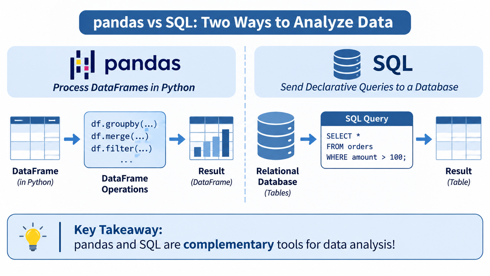
- Context: You know how to manipulate data with Python & pandas. Now let’s explore its database-side counterpart: SQL.
pandas(Python Library):- In-memory dataframes (
pd.DataFrame). - Imperative operations (
df.groupby().mean()). - Great for modeling, machine learning, and visualization.
- In-memory dataframes (
SQL(Database Language):- Client-server / file-based relational databases (SQLite, DuckDB, Postgres).
- Declarative querying (describe what you want, not how to get it).
- Built for storage efficiency, scale, and transaction safety.
pandas vs SQL
Why learn SQL?
- The Real Analyst Workflow: \[\boxed{\text{Business Question} \longrightarrow {\color{blue}{\text{Database Query (SQL)}}} \longrightarrow \text{Query Set} \longrightarrow \text{Analysis / KPI / Model}.}\]
- Enterprise Reality: Most corporate data lives in relational databases or data warehouses (Snowflake, BigQuery, PostgreSQL), not clean CSV files.
- Performance & Scale: SQL databases handle millions of rows efficiently without crashing your local RAM.
- Collaboration:
- Data engineers commonly build databases in SQL
- ata analysts query them to analyze and extract insights.
One dataset, two ways of working
- Let
tablebe the data table, let’s compare common operations across paradigms:
| Operation | pandas (Python) | SQL (RD) |
|---|---|---|
| Select columns | df[['col1', 'col2']] |
SELECT col1, col2 FROM table |
| Filter rows | df[df['age'] > 30] |
SELECT * FROM table WHERE age > 30 |
| Sort values | df.sort_values('date', ascending=False) |
SELECT * FROM table ORDER BY date DESC |
| Aggregate | df.groupby('cat').mean() |
SELECT cat, AVG(val) FROM table GROUP BY cat |
| Join tables | pd.merge(df1, df2, on='id', how='inner') |
SELECT * FROM t1 JOIN t2 ON t1.id = t2.id |
2 Getting Started with SQL
2.1 What is SQL?
- Relational Database Management System (RDBMS):
- Data stored in normalized tables (relations).
- Tables consist of rows (records/entities) and columns (attributes/fields).
- Linked via keys (Primary Keys & Foreign Keys).
  CUSTOMERS TABLE
┌────┬──────────┬───────────┐
│ ID │ Name     │ City      │
├────┼──────────┼───────────┤
│  1 │ Alice    │ Phnom Penh│
│  2 │ Bob      │ Siem Reap │
└────┴──────────┴───────────┘
            │   (1-to-Many)
            ▼
       ORDERS TABLE
┌─────┬─────────────┬────────┐
│ Ord │ Customer_ID │ Amount │
├─────┼─────────────┼────────┤
│ 101 │           1 │  45.50 │
│ 102 │           1 │ 120.00 │
│ 103 │           2 │  15.00 │
└─────┴─────────────┴────────┘- Declarative Nature: You specify what data to retrieve, and the database engine optimizes how to fetch it.
Primary keys: identifier of items/records in entity tables. Foreign key: reference to links of primary keys created in liked tables.
Which platform should we use?
- Low-Friction Classroom Options:
- SQLite Online: Browser-based, zero installation, supports SQLite, PostgreSQL, MySQL, and MS SQL.
- DB Browser for SQLite: Lightweight desktop application for managing local
.dbfiles.
- Production & Big Data Tools:
- DuckDB: In-process analytical database, fantastic companion to Python/pandas.
- PostgreSQL / MySQL: Robust enterprise-grade relational database servers.
Getting started: create a database
- Creating tables using DDL (Data Definition Language):
- Key remark: Unlike pandas where data types are inferred dynamically upon reading a CSV, SQL requires explicit schema definitions and data types (
INTEGER,TEXT,REAL,DATETIME). - Task: Add a few more customers to the
customerstable.
Our running example: a small shop
- We will query a compact shop database containing two related tables:
customers: stores customer profile information (customer_id,name,city,signup_date).orders: stores transaction records (order_id,customer_id,order_date,amount,status).
  CUSTOMERS TABLE
┌────┬──────────┬───────────┐
│ ID │ Name     │ City      │
├────┼──────────┼───────────┤
│  1 │ Alice    │ Phnom Penh│
│  2 │ Bob      │ Siem Reap │
└────┴──────────┴───────────┘
            │   (1-to-Many)
            ▼
       ORDERS TABLE
┌─────┬─────────────┬────────┐
│ Ord │ Customer_ID │ Amount │
├─────┼─────────────┼────────┤
│ 101 │           1 │  45.50 │
│ 102 │           1 │ 120.00 │
│ 103 │           2 │  15.00 │
└─────┴─────────────┴────────┘- Relationship: One customer can place many orders (1-to-Many relationship).
- We will use this running example to master filtering, grouping, joining, and table modification. Task: Create
Orderstable.
3 Database Design & Manipulation
3.1 Flat files to relational tables
- The Problem with Flat Files (Spreadsheets):
- A single giant CSV containing customer details repeated across every single transaction row.
- Consequences:
- Redundant storage space.
- Risk of update anomalies (if a customer changes their city, you must update 50 rows instead of 1).
- Relational Principle (Normalization):
- Split entities into distinct thematic tables.
- Link them using unique identifiers (Keys) to maintain data integrity.
Keys and relationships
- Primary Key (PK):
- A column (or set of columns) that uniquely identifies each row in a table (e.g.,
customer_id). - Must contain unique, non-null values.
- A column (or set of columns) that uniquely identifies each row in a table (e.g.,
- Foreign Key (FK):
- A column in one table that references the Primary Key of another table (e.g.,
orders.customer_idreferencescustomers.customer_id).
- A column in one table that references the Primary Key of another table (e.g.,
- Relationship Types:
- 1-to-Many: One customer has many orders. (Most common).
- 1-to-1: One user profile has one extended passport record.
- Many-to-Many: Students enroll in many courses, courses have many students (requires a junction/bridge table).
Database design: a practical checklist
- Identify Entities: What are the core business objects? (e.g., Customers, Products, Orders, Categories).
- Determine Grain: What does a single row represent? (e.g., One row per order item).
- Define Keys & Constraints: Assign primary keys, foreign keys,
NOT NULL, andUNIQUEconstraints. - Choose Data Types: Match columns to appropriate types (
INTEGER,REAL,TEXT,DATE). - Minimize Redundancy: Avoid storing derived calculations or duplicate descriptive attributes across tables.
Create tables: DDL
- Building a robust table schema with constraints:
--| echo: true
--| code-fold: true
CREATE TABLE products (
    product_id INTEGER PRIMARY KEY,
    product_name TEXT NOT NULL,
    price REAL CHECK(price >= 0),
    category TEXT
);

CREATE TABLE order_items (
    order_id INTEGER,
    product_id INTEGER,
    quantity INTEGER NOT NULL CHECK(quantity > 0),
    PRIMARY KEY (order_id, product_id),
    FOREIGN KEY (order_id) REFERENCES orders(order_id),
    FOREIGN KEY (product_id) REFERENCES products(product_id)
);- Key Concept: Constraints (
CHECK,NOT NULL,FOREIGN KEY) act as automated database guardrails protecting data quality at insertion time.
Insert records: INSERT
- Inserting Single Records:
Persistence: Unlike Python objects stored in volatile RAM, SQL inserts persist data immediately to disk (or secure storage).
Inserting Multiple Rows:
- Comparison: Equivalent to appending rows to a pandas DataFrame using
pd.concat(), but with strict schema enforcement.
Update and delete records
Updating Records (
UPDATE):Deleting Records (
DELETE):
- ⚠️ Critical Danger Warning:
- Omitting the
WHEREclause in anUPDATEorDELETEstatement modifies or deletes every single row in the table! - Always run a corresponding
SELECTstatement with yourWHEREcondition first to verify affected rows.
- Omitting the
Querying vs. changing data
- Overview of SQL Command Categories:
| Category | Description | Key Commands |
|---|---|---|
| DQL (Data Query Language) | Retrieve data from databases | SELECT |
| DDL (Data Definition Language) | Define and modify table structures | CREATE, ALTER, DROP |
| DML (Data Manipulation Language) | Insert, update, and delete records | INSERT, UPDATE, DELETE |
| TCL (Transaction Control Language) | Manage database transactions | COMMIT, ROLLBACK, SAVEPOINT |
4 Querying: SELECT
4.1 The basic SELECT statement
pandas:SQLEquivalent Query:Anatomy:
SELECT: Choose columns.FROM: Specify table source.LIMIT: Restrict output row count.
Filtering rows: WHERE
- Filter rows using comparison and logical operators:
SQL:
- Common Operators in
WHERE:- Logic:
=,!=or<> - Set:
IN('Phnom Penh', 'Siem Reap') - Date:
BETWEEN '2025-01-01' AND '2025-12-31' - Pattern:
LIKE 'Srey%'.
- Logic:
Sorting and limiting
SQL Sorting:
Ordering Rules:
ASC(default): ascending order (\(1 \to 10\), \(A \to Z\)).DESC: descending order (\(10 \to 1\), \(Z \to A\)).- Multiple columns break ties.
Derived columns: expressions and CASE
- Compute calculated fields or categorical labels directly in SQL:
pandasway: Similar tonp.select()or custom lambda functions applied with.apply().- Benefit: Shifts transformation logic to the database layer before transferring data to Python.
- The database engine (
PostgreSQLorSnowflake) handles the computation, reducing data transfer and processing time.
Missing values and NULL
- Checking for NULLs:
- Counting Rules:
COUNT(*)counts all rows (including NULLs).COUNT(column)ignoresNULLvalues in that column.
- Imputation / Fallback:
- pandas Analogies:
df['city'].isna()df['city'].notna()len(df)vsdf['city'].count()df['city'].fillna('Unknown')
- Important: In SQL,
NULLrepresents an unknown or missing value and is never equal to anything—not even anotherNULL.
5 Aggregation & Grouping
5.1 Summary statistics
pandas:
- SQL Aggregate Functions:
COUNT(): Count records.SUM(): Total sum of numeric values.AVG(): Arithmetic mean.MIN()/MAX(): Extrema values.
Grouping: GROUP BY
- Compute group-level metrics by combining
GROUP BYwith aggregate functions:
- pandas:
- Mental Model: Splitting the dataset into partitions, applying calculations independently per partition, and combining results.
- Order:
FROM->GROUP BY->Aggregate Func->SELECT->ORDER BY.
Filter groups: HAVING
The Dilemma: How do we filter based on an aggregated result (like total sales > $500)?
WHEREfilters individual rows before grouping.HAVINGfilters groups after aggregation.
SQL Example:
SQL Clause Execution Order: \[\text{FROM} \longrightarrow \text{WHERE} \longrightarrow \text{GROUP BY} \longrightarrow \text{HAVING} \longrightarrow \text{SELECT} \longrightarrow \text{ORDER BY} \longrightarrow \text{LIMIT}\]
6 Combining Tables: JOIN
6.1 Why do we need JOIN?
CUSTOMERS        ORDERS
┌────┬───────┐   ┌─────┬─────────────┬────────┐
│ id │ name  │   │ ord │ customer_id │ amount │
├────┼───────┤   ├─────┼─────────────┼────────┤
│  1 │ Alice │◄──┤ 101 │           1 │  45.50 │
│  2 │ Bob   │   │ 102 │           2 │ 120.00 │
└────┴───────┘   └─────┴─────────────┴────────┘
▲ (matched on customer_id)- Normalized Database Design:
- Storing customer names and cities repeatedly inside every single order record causes data redundancy.
- Instead, we split entities into separate tables:
customersandorders.
- The Challenge: How do we analyze customer purchasing behavior across both tables simultaneously?
- The Solution: Relational
JOINoperations using matching keys (customer_id).
INNER JOIN and LEFT JOIN
INNER JOIN: Returns only rows with matching keys in both tables.
(Drops customers with zero orders and orders with invalid customer IDs).
customers candorders oassign short aliases to the tables to easily access their columns.
JOIN compared with pandas merge
- Mapping SQL join types directly to pandas syntax:
| Join Type | SQL Syntax | pandas Equivalent |
|---|---|---|
| Inner Join | FROM t1 JOIN t2 ON ... |
pd.merge(t1, t2, how='inner', on='id') |
| Left Join | FROM t1 LEFT JOIN t2 ON ... |
pd.merge(t1, t2, how='left', on='id') |
| Right Join | FROM t1 RIGHT JOIN t2 ON ... |
pd.merge(t1, t2, how='right', on='id') |
| Outer Join | FROM t1 FULL OUTER JOIN t2 ON ... |
pd.merge(t1, t2, how='outer', on='id') |
7 Validation & Practical Workflow
7.1 Validate your query results
- Q: How do we verify our SQL queries are correct and bug-free?
- Validation Checklist:
- Row Count Checks: Did your
JOINunexpectedly multiply rows (cartesian explosion)? CheckCOUNT(*)before and after joins. - Key Uniqueness: Verify primary keys have zero duplicates (
SELECT id, COUNT(*) FROM t GROUP BY id HAVING COUNT(*) > 1). - Missing Values: Check for unexpected
NULLvalues resulting from unmatched left joins (WHERE col IS NULL). - Totals & Sanity Checks: Compare aggregated sum totals against raw table summaries.
- Row Count Checks: Did your
- If results look anomalous, flag 🚩 the query and investigate the underlying data grain!
A typical SQL workflow
- Clarify Question: Translate business objectives into analytical requirements.
- Inspect Tables: Identify relevant tables, schemas, and primary/foreign keys.
- Draft Select & Filter: Write base queries using
SELECT,WHERE, andLIMIT. - Aggregate & Group: Apply summary metrics using
GROUP BYandHAVING. - Join Entities: Combine related tables via
INNER JOINorLEFT JOIN. - Validate Results: Check row counts, handle nulls, and verify totals.
- Communicate Insights: Export results or pass dataframes to Python for visualization.
Summary
- SQL vs pandas: SQL is declarative and database-native, designed for scalable querying; pandas is imperative and in-memory, ideal for Python modeling.
- Master the SELECT Pipeline: Combine
SELECT,WHERE,ORDER BY, andLIMITto filter and sort data efficiently. - Aggregation & Grouping: Use
GROUP BYfor partition summaries andHAVINGto filter aggregated groups. - Relational Joins: Connect normalized tables using
INNER JOINandLEFT JOINmatching keys. - Database Design & DML: Enforce structure with DDL constraints and modify data safely using
INSERT,UPDATE, andDELETE. - Always Validate: Rigorously check row counts, keys, and totals at every step of your analytical workflow.
🥳 Yeahhhh 🥂!!!
Any question? Else, we take a break!
🥳 Yeahhhh 🥂!!!
Let’s take a break!
