
| latitude | total_rooms | population | median_income | median_house_value | ocean_proximity | |
|---|---|---|---|---|---|---|
| 0 | 37.88 | 880.0 | 322.0 | 8.3252 | 452600.0 | NEAR BAY |
| 1 | 37.86 | 7099.0 | 2401.0 | 8.3014 | 358500.0 | NEAR BAY |
| 2 | 37.85 | 1467.0 | 496.0 | 7.2574 | 352100.0 | NEAR BAY |
| 3 | 37.85 | 1274.0 | 558.0 | 5.6431 | 341300.0 | NEAR BAY |
| 4 | 37.85 | 1627.0 | 565.0 | 3.8462 | 342200.0 | NEAR BAY |
Dimensional reduction: PCA & t-SNE
INS-605: Data Analysis II

Lecturer: Dr. Sothea HAS
Helpful resources
1 Motivation
1.1 Motivation
California Housing Prices dataset
- The data contains information of neighborhoods from the 1990 California census.
- Dimension: (20640, 10).
- How are the
sizeandeconomicof neighborhoods related? - How are the previous related to their locations?
1.2 Compression Signal
- Correlation matrix summarizes the similarity of the columns.
- Many correlated columns, better column reduction.
2 Principal Directions (PDs) & Components (PCs)
2.1 PCA Concept
Why reducing dimension?
- High-dimensional data: “large number of columns/fat data”.
- There are many problems when dealing with high-dimensional data:
- Curse of dimensionality
- Complexity: analysis and computation
- Cannot be visualized
- Noise & prone to overfitting…
- The core idea that makes “Dimensional Reduction” possible is that HD data often live in smaller dimensional spaces.

- PCA works by rotating the data in a way that the new columns are orthogonal and capture the most variance.
2.2 PDs & PCs
Principal Directions (PDs)
- Given data matrix: \(D\in\mathbb{R}^{n\times d}\),
| X | Y | Z | |
|---|---|---|---|
| 0 | 0.041 | 1.192 | 1.591 |
| 1 | -1.439 | 2.870 | 1.992 |
| 2 | 1.661 | 2.043 | 4.787 |
| 3 | -2.891 | 0.794 | -1.043 |
| 4 | 1.618 | 3.229 | 3.470 |
| 5 | 2.310 | 2.082 | 3.454 |
Principal Directions (PDs)
- Principal Directions (PDs) are the most important directions in PCA.
Definition: Principal Directions \(\vec{u}_k\)
- The 1st Principal Direction (PD) \(\color{red}{\vec{u}_1}\in\mathbb{R}^d\) is the unit vector or direction that the data spreads or varies the most: \(\color{red}{\vec{u}_1}=\arg\max_{\vec{u}\in\mathbb{R}^d:\|\vec{u}\|^2=1}\|D\color{purple}{\vec{u}}\|^2.\)
- The 2nd PD \(\color{green}{\vec{u}_2}\in\mathbb{R}^d\) is the unit direction perpendicular to \(\color{red}{\vec{u}_1}\) and captures 2nd largest variation of the data: \(\color{green}{\vec{u}_2}=\arg\max_{\vec{u}\in\mathbb{R}^d:\|\color{purple}{\vec{u}}\|^2=1,\color{purple}{\vec{u}}\perp \color{red}{\vec{u}_1}}\|D\color{purple}{\vec{u}}\|^2.\)
- The \(k\)-th PD \(\color{blue}{\vec{u}_k}\in\mathbb{R}^d\) (\(3\leq k\leq d\)) is the unit direction that is perpendicular to \(S_{k-1}=\{\color{red}{\vec{u}_1},\color{green}{\vec{u}_2},\dots,\color{purple}{\vec{u}_{k-1}}\}\) and captures the \(k\)-th largest variation of the data: \(\color{blue}{\vec{u}_k}=\arg\max_{\color{purple}{\vec{u}}\in\mathbb{R}^d:\|\color{purple}{\vec{u}}\|^2=1,\color{purple}{\vec{u}}\perp S_{k-1}}\|D\color{purple}{\vec{u}}\|^2.\)
Principal Components (PCs)
- Principal Directions (PDs) are the most important directions in PCA.
Definition: Principal Components \(\text{PC}_j\)
- Let \(\color{blue}{U}\) be a \(d\times d\) matrix with all PDs columns, i.e., \[\color{blue}{U}=[\color{red}{\vec{u}_1}|\color{green}{\vec{u}_2}|\dots |\color{blue}{\vec{u}_d}],\] then \(\color{red}{\tilde{D}}=D\color{blue}{U}\) is the rotated data with the following properties:
- Independent cols: \(\color{blue}{\tilde{D_j}}\perp \color{blue}{\tilde{D_k},\forall j\neq k}\).
- For any \(j=1,2,...,d:\color{blue}{\tilde{D_j}}\) is the column with \(j\)-th largest variation.
- Total var: \(\sum_{j=1}^d\|\color{blue}{\tilde{D_j}}\|^2=\sum_{j=1}^d\|D_j\|^2.\)
- The columns \(\color{blue}{\tilde{D_j}}\)’s are called Principal Components (PCs) of \(D\) denoted by \(\color{blue}{\text{PC}_j}\).
How to find PDs & PCs
- Perform PCA comes down to computing rotated data \(\color{red}{\tilde{D}}=D\color{blue}{U}\) or computing \(\color{blue}{U}\).
Principal Direction Solution
- Without loss of generality, we assume that the data is centered (\(\overline{D}_j=0\),\(\forall j=1,\dots,d\)).
- The 1st PD \(\color{red}{\vec{u}_1}\) is the eigenvector of matrix \(A=D^TD\) with the largest eigenvalue \(\color{red}{\lambda_1}\geq 0\), i.e., \((\color{red}{\vec{u}_1},\color{red}{\lambda_1})\) solves \(A\color{red}{\vec{u}_1}=\color{red}{\lambda_1\vec{u}_1}\).
- The 2nd PD \(\color{green}{\vec{u}_2}\) is the eigenvector of matrix \(A=D^TD\) with the 2nd largest eigenvalue \(\color{green}{\lambda_2}\geq 0\), i.e., \((\color{green}{\vec{u}_2},\color{green}{\lambda_2})\) solves \(A\color{green}{\vec{u}_2}=\color{green}{\lambda_2\vec{u}_2}\).
- The \(k\)-th PD \(\color{blue}{\vec{u}_k}\) is the eigenvector of matrix \(A=D^TD\) with the \(k\)-th largest eigenvalue \(\color{blue}{\lambda_k}\geq 0\), i.e., \((\color{blue}{\vec{u}_k},\color{blue}{\lambda_k})\) solves \(A\color{blue}{\vec{u}_k}=\color{blue}{\lambda_k\vec{u}_k}\).
Solution to Principal Directions \(\vec{u}_k\)
- PDs \(\color{red}{\vec{u}_1},\dots,\color{blue}{\vec{u}_d}\) are the 1st, …, \(d\)-th eigenvectors of matrix \(A=D^TD\) with eigenvalues \(\color{red}{\lambda_1}\geq\dots\geq\color{blue}{\lambda_d}\geq 0\) respectively.
- Principal components are the columns of
\[\begin{align*} \underbrace{\color{red}{\tilde{D}}}_{n\times d}&=\underbrace{D}_{n\times d}\times\underbrace{\color{blue}{U}}_{n\times d}\\ &=\begin{bmatrix} x_{11} & \dots & x_{1d}\\ x_{21} & \dots & x_{2d}\\ x_{31} & \dots & x_{3d}\\ \vdots & \ddots & \vdots\\ x_{n1} & \dots & x_{nd}\end{bmatrix} \begin{bmatrix} \color{red}{u_{11}} & \dots & \color{blue}{u_{1d}}\\ \color{red}{u_{21}} & \dots & \color{blue}{u_{2d}}\\ \vdots & \ddots & \vdots\\ \color{red}{u_{d1}} & \dots & \color{blue}{u_{dd}}\end{bmatrix} \end{align*}\]
- The \(\color{blue}{\text{PC}_j}\) is the combination of original columns of \(D_k\)’s, i.e., \(\color{blue}{\text{PC}_j}=\sum_{k=1}^du_{kj}D_k.\)
Implementation of PCA
Unnormalized PCA
- Given data: \(D\in\mathbb{R}^{n\times d}\)
- Centering \(D_c=\underbrace{D}_{n\times d} -\underbrace{\mathbb{1}_n}_{n\times n}\overbrace{D}^{n\times d}/n.\)
- Perform Eigenvalue Decomposition on covariance matrix \(V=D_c^TD_c/(n-1)\), i.e., \[V=\color{blue}{U}\Lambda \color{blue}{U}^T,\]
- \(\color{blue}{U}\): matrix of eigenvectors
- \(\Lambda=\text{diag}(\color{red}{\lambda_1},\dots,\color{blue}{\lambda_d})\): diagonal matrix of eigenvalues \(\color{red}{\lambda_1}\geq \dots\geq \color{blue}{\lambda_d}\geq 0\).
Normalized PCA
- Given data: \(D\in\mathbb{R}^{n\times d}\)
- Standardizing: compute std matrix \(\color{red}{\Sigma}=\text{diag}(\widehat{\sigma}_1,\dots,\widehat{\sigma}_d)\) and standardized data \(Z=(\underbrace{D}_{n\times d} -\underbrace{\mathbb{1}_n}_{n\times n}\overbrace{D}^{n\times d}/n)\color{red}{\Sigma^{-1}}.\)
- Perform Eigenvalue Decomposition on correlation matrix \(C=Z^TZ/(n-1)\), i.e., \[C=\color{blue}{U}\Lambda \color{blue}{U}^T.\]
- Rotated data: \(\color{red}{\tilde{D}}=D\color{blue}{U}.\) [👉 Demo]
Geometric Interpretation of PCA
3 Dimensional Reduction Reconstruction
3.1 Reduction/Reconstruction
Dimensional Reduction
- Reduction to \(\color{red}{k}<d\) dimensions is done by \(\color{red}{\tilde{D}_k}=\color{red}{\tilde{D}}[:,:\color{red}{k}].\)
- Quality of representation on each direction: \(\left[\frac{\lambda_1}{\sum_{j=1}^d\lambda_j},\dots,\frac{\lambda_{\color{red}{k}}}{\sum_{j=1}^d\lambda_j}\right].\)
- Variance explained by \(\color{red}{k}\) dimensions: \(\frac{\sum_{j=1}^{\color{red}{k}}\lambda_j}{\sum_{j=1}^d\lambda_j}\times 100.\)
- For visualization, one can choose \(\color{red}{k}=2\) or \(3\). [👉 Demo]
* Total variation of X: 17.79| X | Y | Z | |
|---|---|---|---|
| 0 | 0.041 | 1.192 | 1.591 |
| 1 | -1.439 | 2.870 | 1.992 |
| 2 | 1.661 | 2.043 | 4.787 |
| 3 | -2.891 | 0.794 | -1.043 |
| 4 | 1.618 | 3.229 | 3.470 |
* Total variation of proj: 15.2| PC1 | PC2 | PC3 | |
|---|---|---|---|
| 0 | -2.424 | -0.173 | -0.197 |
| 1 | -2.287 | 2.086 | -0.406 |
| 2 | 1.239 | -0.292 | -0.558 |
| 3 | -6.119 | 1.163 | -0.709 |
| 4 | 0.509 | 0.555 | 0.818 |
Dimensional Reduction
- Reduction to \(\color{red}{k}<d\) dimensions is done by \(\color{red}{\tilde{D}_k}=\color{red}{\tilde{D}}[:,:\color{red}{k}].\)
- Quality of representation on each direction: \(\left[\frac{\lambda_1}{\sum_{j=1}^d\lambda_j},\dots,\frac{\lambda_{\color{red}{k}}}{\sum_{j=1}^d\lambda_j}\right].\)
- Variance explained by \(\color{red}{k}\) dimensions: \(\frac{\sum_{j=1}^{\color{red}{k}}\lambda_j}{\sum_{j=1}^d\lambda_j}\times 100.\)
- For visualization, one can choose \(\color{red}{k}=2\) or \(3\). [👉 Demo]
- Application on California Housing:
- Variance explained by 2 PCs: 79.86%.
Dimensional Reduction
- Reduction to \(\color{red}{k}<d\) dimensions is done by \(\color{red}{\tilde{D}_k}=\color{red}{\tilde{D}}[:,:\color{red}{k}].\)
- Quality of representation on each direction: \(\left[\frac{\lambda_1}{\sum_{j=1}^d\lambda_j},\dots,\frac{\lambda_{\color{red}{k}}}{\sum_{j=1}^d\lambda_j}\right].\)
- Variance explained by \(\color{red}{k}\) dimensions: \(\frac{\sum_{j=1}^{\color{red}{k}}\lambda_j}{\sum_{j=1}^d\lambda_j}\times 100.\)
- For visualization, one can choose \(\color{red}{k}=2\) or \(3\). [👉 Demo]
Reconstruction
- The reconsution is defined by: \[\color{green}{D_k^{\text{rec}}}=\color{red}{\tilde{D}_k}\color{blue}{U[:,:k]^T}.\]
- Low-rank approximation shows that this reconstruction \(\color{green}{D_k^{\text{rec}}}\) is the best \(k\)-rank approximation of \(D\) w.r.t. Frobenius norm, i.e., \[\color{green}{D_k^{\text{rec}}}=\arg\min_{M_k:r(M_k)\leq k}\|X-M_k\|_F,\] where \(\|D\|_F=\sqrt{\sum_{i,j}D_{ij}^2}\) is the Frobenius norm.
Summary
PCAcaptures and arranges directions with largest, 2nd largest,… variation into the 1st, 2nd, … column using Spectral Theorem (Eigenvalue decomposition).- These directions are contained in the eigenvector matrix of Covariance (unnormalized) or Correlation matrix (normalized) of the data.
- The variation along each direction is given by the corresponding eigenvalues: \(\lambda_1>\dots>\lambda_d\).
- Our goal is to explore dimensional reduction and reconstruction power of
PCA, however, it can be used in Data Analysis, EDA, Data Summary… - Remark: Many highly correlated columns indicates effective dimensional reduction (the first two PCs can capture significant variation).
4 Correlation Circle
4.1 Correlation Circles
- Besides dimensional reduction,
PCAcan also be used to summarize data.
- How would you explain this graph?
- 🔑 The connection between PCs and the original columns.
- Correlation Circle is the key.
- One can compute correlations between original data with PCs:
Code
| PC1 | PC2 | |
|---|---|---|
| housing_median_age | -0.426668 | 0.048696 |
| total_rooms | 0.963481 | 0.087248 |
| total_bedrooms | 0.971857 | -0.077096 |
| population | 0.930272 | -0.113646 |
| households | 0.975068 | -0.059403 |
| median_income | 0.107198 | 0.912892 |
| median_house_value | 0.084727 | 0.913812 |
Code
fig_cir = go.Figure()
circle = go.Scatter(
    x=np.cos(np.linspace(0, 2 * np.pi, 100)),
    y=np.sin(np.linspace(0, 2 * np.pi, 100)),
    mode='lines',
    name='Unit Circle',
    line=dict(color='black', dash='dash')
)
fig_cir.add_trace(circle)
fig_cir.add_trace(go.Scatter(
    x=[-1,1],
    y = [0,0],
    mode="lines", line=dict(color='black', dash='dash')
))
fig_cir.add_trace(go.Scatter(
    x=[0,0],
    y = [-1,1],
    mode="lines", line=dict(color='black', dash='dash')
))

loc = ['top right', 'top left', 'bottom right', 'bottom left', 'top right', 'top left', 'bottom right']

# Add loading vectors
for i, feature in enumerate(quan_cols[2:]):
    fig_cir.add_trace(go.Scatter(
        x=[0, Corr_matrix.iloc[i, 0]],
        y=[0, Corr_matrix.iloc[i, 1]],
        mode='lines+text',
        text=[None, feature],
        textposition=[loc[i]],
        name=feature,
        showlegend=True
    ))

# Set the layout
fig_cir.update_layout(
    {'paper_bgcolor': 'rgba(0,0,0,0)',
    'plot_bgcolor': 'rgba(0,0,0,0)'},
    title='Correlation Circle',
    xaxis=dict(title='PC1 ('+str(np.round(pca.explained_variance_ratio_[0]*100,2)) + '%)', range=[-1.2, 1.2]),
    yaxis=dict(title='PC2 ('+str(np.round(pca.explained_variance_ratio_[1]*100,2)) + '%)', range=[-1.2, 1.2]),
    showlegend=False,
    width=400,
    height=400
)
fig_cir.update_xaxes(
    showline=True,
    linewidth=1,
    linecolor='gray',
    mirror=True,  # Mirrors the bottom x-axis line to the top
    showgrid=True, gridwidth=1, gridcolor=LIGHT_GRAY
)
fig_cir.update_yaxes(
    showline=True,
    linewidth=1,
    linecolor='gray',
    mirror=True,  # Mirrors the left y-axis line to the right
    showgrid=True, gridwidth=1, gridcolor=LIGHT_GRAY
)
fig_cir.show()
Interpretation
- Long variables indicate large correlation with the PCs therefore well represented by the PCs.
- Highly correlated original variables are mostly aligned.
- Those that are nearly perpendicular, tend to be decorrelated.
- PC1 is strong related to neighborhood size variables.
- PC2 is strong reated to financial condition variables.
- Correlation circles can be used to summarize the Biplot of individuals.
- Correlation circles can summarize the relationship between original variables, between original variables and PCs and help interpreting the Biplot.
- ⚠️ Caution: Interpretation of PCs may be misleading! It’s intuition not the fact!
5 t-Stochastic Neighbor Embedding (t-SNE)
5.1 t-SNE
- Let \(X\in\mathbb{R}^{n\times d}\) with large \(d\).
Objective
\(t\)-SNE aims at finding lower dimensional (LD) representation of \(X\) (2 or 3) so that the distribution among LD data is similar to the original data.
- Hinton and Roweis (2002) proposed Stochastic Embedding Neighbor (SNE).
- \(t\)-SNE is the improved version [see Laurens, \(t\)-SNE Page].
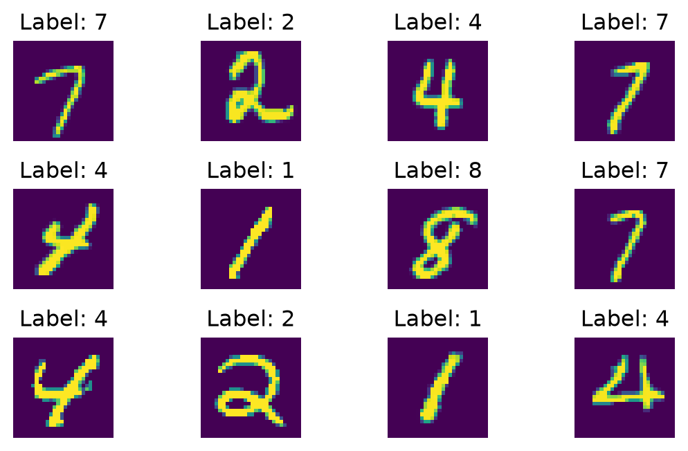
Code
from sklearn.manifold import TSNE

# Prepare the t-SNE model
tsne = TSNE(n_components=2, random_state=42)

# Fit and transform the data
X_tsne = tsne.fit_transform(X[:1000,:])  # Use a subset for faster computation
df_tsne = pd.DataFrame(X_tsne, columns=['Component 1', 'Component 2'])
df_tsne['label'] = y_train[:1000]
fig_tsne = px.scatter(df_tsne, x="Component 1", y="Component 2", color="label")
fig_tsne.update_layout(height=420, width=550, title="t-SNE visualization on MNIST")
fig_tsne.show()
Original & embedding data in \(t\)-SNE
- Pairwise similarities in the original space:
- Conditional probabilities (Gaussian): prob. that \(\text{x}_j\) is a neighbor of \(\color{purple}{\text{x}_i}\in\mathbb{R}^d\): \[p_{j|\color{purple}{i}}=\frac{e^{-\|\text{x}_j-\color{purple}{\text{x}_i}\|^2/(2\sigma_{\color{purple}{i}}^2)}}{\sum_{k\neq \color{purple}{i}}^n e^{-\|\text{x}_k-\color{purple}{\text{x}_i}\|^2/(2\sigma_{\color{purple}{i}}^2)}}\] with \(\sigma_{\color{purple}{i}}>0\) defines the crowd around \(\color{purple}{\text{x}_i}\).
- Symmetric probs: \(\displaystyle \color{blue}{p_{i,j}}=\frac{p_{j|\color{purple}{i}}+p_{i|\color{purple}{j}}}{2n}.\) \[\color{blue}{P} = \begin{bmatrix}\color{blue}{p_{1,1}} & \color{blue}{p_{1,2}} & \color{blue}{...} & \color{blue}{p_{1,n}}\\ \color{blue}{p_{2,1}} & \color{blue}{p_{2,2}} & \color{blue}{...} & \color{blue}{p_{2,n}}\\ \color{blue}{\vdots} & \color{blue}{\vdots} & \color{blue}{\ddots} & \color{blue}{\vdots}\\ \color{blue}{p_{n,1}} & \color{blue}{p_{n,2}} & \color{blue}{...} & \color{blue}{p_{n,n}}\end{bmatrix}\]
- Objective of \(t\)-SNE: find low-dimensional data points \(\color{red}{\text{z}_1},\dots, \color{red}{\text{z}_n}\in\mathbb{R}^{d'}\) (\(d'<d\)) distributing according to the original data structure i.e., preserving the pairwise similarities.
- \(t\)-distribution probabilities between embedded data points \(\color{red}{\text{z}_i,\text{z}_j}\in\mathbb{R}^{d'}\): \[\color{red}{q_{i,j}}=\frac{(1+\|\text{z}_i-\text{z}_j\|^2)^{-1}}{\sum_{k\neq \ell:k,\ell=1}^n (1+\|\text{z}_k-\text{z}_{\ell}\|^2)^{-1}}.\] \[\color{red}{Q} = \begin{bmatrix}\color{red}{q_{1,1}} & \color{red}{q_{1,2}} & \color{red}{...} & \color{red}{q_{1,n}}\\ \color{red}{q_{2,1}} & \color{red}{q_{2,2}} & \color{red}{...} & \color{red}{q_{2,n}}\\ \color{red}{\vdots} & \color{red}{\vdots} & \color{red}{\ddots} & \color{red}{\vdots}\\ \color{red}{q_{n,1}} & \color{red}{q_{n,2}} & \color{red}{...} & \color{red}{q_{n,n}}\end{bmatrix}\]
- We want to learn \((\color{red}{z_i})\) by minimizing the distance between \(\color{red}{Q}\) and \(\color{blue}{P}\).
Optimization for LD data \(\color{red}{z_i}\)
- In the first proposed method (SNE in Hinton and Roweis (2002)), \(\color{red}{q_{i,j}}\) was also Gaussian similarity. This often leads to Crowding Problem.
- Solution: \(t\)-distribution provides better shape for similarity in LD space because of its heavy tail.
- \(t\)-SNE optimization: force LD data structure \(\color{red}{Q=(q_{i,j})}\) to be similar to original data structure \(\color{blue}{P=(p_{i,j})}\) using Kullback-Leibler divergence: \[D_{KL}(\color{blue}{P}||\color{red}{Q})=\sum_{i,j}\color{blue}{p_{i,j}}\log\left(\frac{\color{blue}{p_{i,j}}}{\color{red}{q_{i,j}}}\right).\]
- Gradient of KL w.r.t \(z_i\):
\[\frac{\partial KL}{\partial \color{red}{z_{i}}}=4\sum_{j}(\color{blue}{p_{i,j}}-\color{red}{q_{i,j}})(\color{red}{z_{i}}-\color{red}{z_{j}})(1+\|\color{red}{z_{i}}-\color{red}{z_{j}}\|^2)^{-1}.\]
Gradient Descent With Momentum
- Data: \(X=\{\text{x}_1,\dots,\text{x}_n\}\).
- Perplexity: Perp (effective local neighbors between 5 and 50).
- Parameters:
max_iter, learning rate: \(\eta\), momentum \(\alpha(t)\). - Result: LD data \(Z=\{z_1,\dots,z_n\}\).
- Begin:
- Compute \(p_{i,j}\)
- Initialize: \(Z^{(0)}=\{z_1^{(0)},\dots,z_n^{(0)}\}\)
for t=1 to max_iter do:- Compute \(q_{i,j}\) and gradient: \(\frac{\partial KL}{\partial z_i}\)
- Update: \(Z^{(t)}=Z^{(t-1)}-\eta\frac{\partial KL}{\partial z_i}+\alpha(t)(Z^{(t-1)}-Z^{(t-2)})\).
- End. [👉 Demo]
Use t-SNE effectively, Wattenberg, et al. (2016)
Summary
- \(t\)-SNE is a non-linear dimentional reduction technique aiming at searching for neighbors of points in a lower-dimensional space (2 or 3) especially for visualization.
- High-dimensional data \(X\) is converted to pairwise similarity probability \(\color{blue}{P=(p_{i,j})}\) according to how close they are.
- The pairwise similarity probability \(\color{red}{Q=(q_{i,j})}\) of low-dimensional data points is defined based on \(t\)-distribution of degree 1 or Cauchy distribution.
- The proximity between \(\color{blue}{P}\) and \(\color{red}{Q}\) is measured using KL divergence.
- The LD data \(z_i\) are estimated by minimizing KL divergence using Gradient Descent with Momontum.
- Understand more about \(t\)-SNE: Laurens van der Maaten’s t-SNE Page and How to Use t-SNE Effectively, Distill, Google Brain Team.
🥳 Yeahhhh 🥂!!!
Let’s take a break!
