Generalized Linear Models


INS-605: Data Analysis II

Lecturer: Dr. Sothea HAS

helpful resources

🌐 Generalized Linear Models 2nd Edition by P. McCullagh & J.A. Nelder FRS (1983).

What You Will Learn

By the end of this section, you should be able to:

  1. Explain the structure of linear, logistic, and Poisson regression.
  2. Construct a linear predictor \(\widehat{y}_i=\beta_0+\beta_1x_{i1}+\cdots+\beta_dx_{id}.\)
  3. Use a link function to connect the response to the linear predictor.
  4. Derive the appropriate loss function from the assumed distribution of \(Y\).
  5. Interpret coefficients for:
    • Continuous outcomes,
    • Binary outcomes,
    • Count outcomes.
  6. Perform statistical tests and confidence interval analysis.
  7. Recognize appropriate applications of each model.

1 Multiple Linear Regression (MLR)

1.1 MLR Recap

CRIM INDUS RM AGE TAX PTRATIO LSTAT MEDV
0 0.00632 2.31 6.575 65.2 296.0 15.3 4.98 24.0
1 0.02731 7.07 6.421 78.9 242.0 17.8 9.14 21.6
2 0.02729 7.07 7.185 61.1 242.0 17.8 4.03 34.7
3 0.03237 2.18 6.998 45.8 222.0 18.7 2.94 33.4
4 0.06905 2.18 7.147 54.2 222.0 18.7 5.33 36.2
  • CRIM: Per Capita Crime Rate by town
  • INDUS: Proportion of Non-retail Business acres per town
  • RM: Average Number of Rooms per dwelling
  • AGE: Proportion of Owner-occupied units built prior to 1940
  • TAX: Full-value Property-tax rate per 10,000 dollars
  • PTRATIO: Pupil-Teacher Ratio by town
  • LSTAT: Percentage Lower Status of the Population
  • MEDV: Median value of owner-occupied homes in $1000.
  • Notation:
    • Individual features: \(\underbrace{\text{x}_i}_{[1,\text{features}_i]}\in\mathbb{R}^{d+1}\)
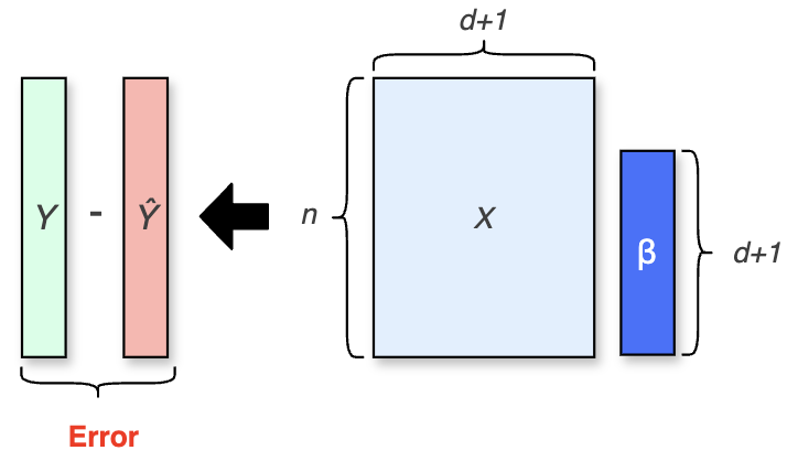
    • Design matrix of features: \({X}\in\mathbb{R}^{n\times (d+1)}\)
    • Individual target/output: \({y_i}\in\mathbb{R}\),
    • Vector of target: \({Y}\in\mathbb{R}^{n}\).
  • Model’s coefficients: \({\color{blue}{\beta}}=[{\color{blue}{\beta_0,\dots,\beta_d}}]\in\mathbb{R}^{d+1}\)
    • Predicted point: \({\color{red}{\widehat{y}_i}}=\text{x}_i^T{\color{blue}{\beta}}\in\mathbb{R}\)
    • Predicted Vector: \({\color{red}{\widehat{Y}}}=\text{X}{\color{blue}{\beta}}\in\mathbb{R}^n\).
    • Residual/error: \({\color{red}{e}_i}=y_i-{\color{red}{\widehat{y}_i}}\)
Gaussian Linear Model Assumption: \[{\color{red}{e}_i}\overset{\text{iid}}{\sim}{\cal N}(0,{\color{blue}{\sigma^2}})\text{ for all }i=1,2,\dots,n,\] for some fixed std \(\color{blue}{\sigma}>0.\)

  • The residual should be centered around 0 with constant variance.

1.1 MLR Recap

  • Ordinary Least Square Goal: Find the best \({\color{blue}{\widehat{\beta}^*}}\) by minimizing Residual Sum of Squares (RSS): \[\boxed{{\color{blue}{\widehat{\beta}^*}}=\arg\min_{\color{blue}{\beta}}\sum_{i=1}^2(y_i-\text{x}_i^T{\color{blue}{\beta}})^2=\|Y-X{\color{blue}{\beta}}\|^2.}\]
  • You can check why \(\color{blue}{\beta}\) is chosen this way! \[\boxed{\text{Min. }{\color{red}{\text{RSS}}}\Leftrightarrow\text{ Max. log-likelihood of data}.}\]
  • Hint: \({\color{red}{e}_i}=y_i-{\color{red}{\widehat{y}_i}}\sim{\cal N}(0,{\color{blue}{\sigma^2}})\) for all \(i\).
    • Step 1: write log-likelihood of \({\color{red}{e}_i}\)’s.
    • Step 2: maximize LLH w.r.t. \(\color{blue}{\beta}\).
  • Many other loss functions in ML are derived this way!
  • Notation:
    • Individual features: \(\underbrace{\text{x}_i}_{[1,\text{features}_i]}\in\mathbb{R}^{d+1}\)
    • Design matrix of features: \({X}\in\mathbb{R}^{n\times (d+1)}\)
    • Individual target/output: \({y_i}\in\mathbb{R}\),
    • Vector of target: \({Y}\in\mathbb{R}^{n}\).
  • Model’s coefficients: \({\color{blue}{\beta}}=[{\color{blue}{\beta_0,\dots,\beta_d}}]\in\mathbb{R}^{d+1}\)
    • Predicted point: \({\color{red}{\widehat{y}_i}}=\text{x}_i^T{\color{blue}{\beta}}\in\mathbb{R}\)
    • Predicted Vector: \({\color{red}{\widehat{Y}}}=\text{X}{\color{blue}{\beta}}\in\mathbb{R}^n\).
    • Residual/error: \({\color{red}{e}_i}=y_i-{\color{red}{\widehat{y}_i}}\)

Gaussian Linear Model Assumption: \[{\color{red}{e}_i}\overset{\text{iid}}{\sim}{\cal N}(0,{\color{blue}{\sigma^2}})\text{ for all }i=1,2,\dots,n,\] for some fixed std \(\color{blue}{\sigma}>0.\)

  • The residual should be centered around 0 with constant variance.

For some details, read Chapter 1: The Gaussian Linear Model

Visualize RSS

1.2 A different view of LM

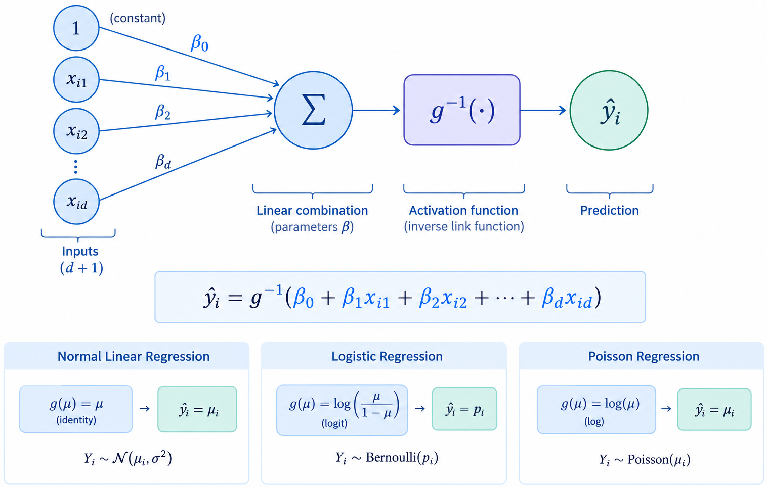
  • We can view Linear Model as a simple neural network:
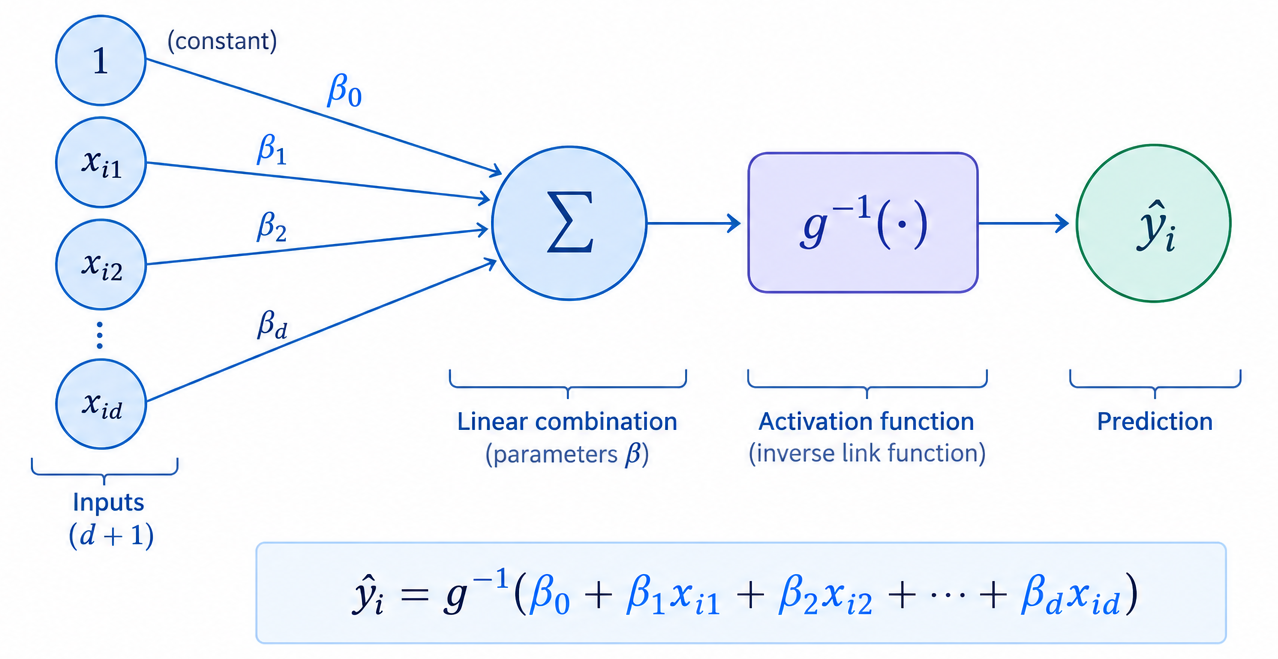
  • \(g^{-1}\) is called activation function in ML, but called inverse link function in statistical learning.
  • GLM is all about using suitable \(g\) for the corresponding target \(Y\).

Real Target: Multiple Linear Regression

  • For GLR (the target \(y_i\in\mathbb{R}\)) for a fixed input \(\text{x}_i\in\mathbb{R}^{d+1}\): \[\begin{align*}{\color{red}{e_i}}&=y_i-{\color{red}{\widehat{y}_i}}\sim{\cal N}(0,{\color{blue}{\sigma^2}})\\ \Leftrightarrow y_i&={\color{red}{\widehat{y}_i}}+{\color{red}{e_i}}\sim{\cal N}({\color{red}{\widehat{y}_i}},{\color{blue}{\sigma^2}})\\ \Rightarrow \mathbb{E}[y_i\mid \text{x}_i]&={\color{red}{\widehat{y}_i}}=\text{x}_i^T{\color{blue}{\beta}}\text{ (also a real number)}.\end{align*}\]

Link Function

  • A Link Function \(g\) is used for converting the average value of the target \(\mu_i=\mathbb{E}[y_i\mid \text{x}_i]\) to match the range of \({\color{red}{\widehat{y}_i}}=\text{x}_i^T{\color{blue}{\beta}}\in\mathbb{R}\), i.e., \[g(\mu_i)={\color{red}{\widehat{y}_i}}=\text{x}_i^T{\color{blue}{\beta}}\text{ or }\mu_i=g^{-1}(\text{x}_i^T{\color{blue}{\beta}}).\]
  • This means that for GLM, \(g(\mu)=\mu\) or \(g^{-1}(\mu)=\mu\) (identity).

Real Target: Interpretation of \({\color{blue}{\beta}}\) in MLR

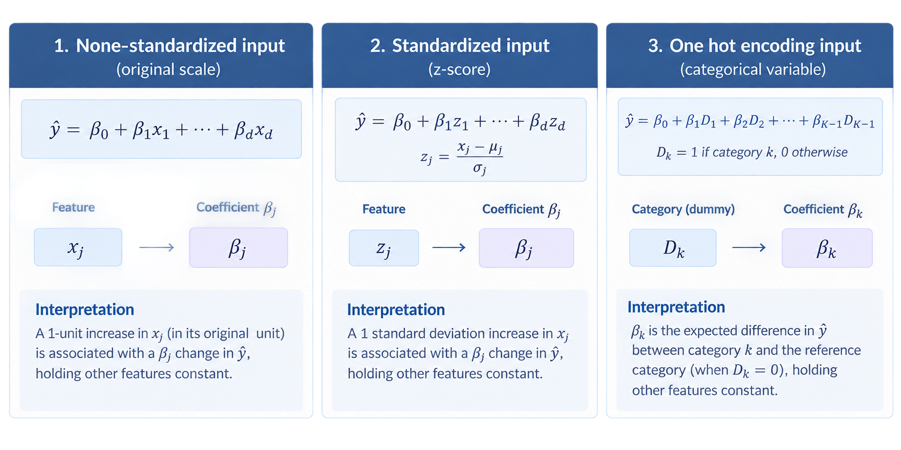
  • MLR is widely used due to its interpretability and transparency. \[ y={\color{blue}{\beta_0}} + {\color{blue}{\beta_1}}\text{x}_1 + \cdots + {\color{blue}{\beta_d}}\text{x}_d + {\color{red}{e}}=\text{x}^T{\color{blue}{\beta}}+{\color{red}{e}}.\]
1.3 Application on MDEV dataset

  • Pearson corr:
Code
df = data.iloc[:,[0,2,5,6,9,10,12,13]]
df.corr().round(2)
CRIM INDUS RM AGE TAX PTRATIO LSTAT MEDV
CRIM 1.00 0.41 -0.22 0.35 0.58 0.29 0.46 -0.39
INDUS 0.41 1.00 -0.39 0.64 0.72 0.38 0.60 -0.48
RM -0.22 -0.39 1.00 -0.24 -0.29 -0.36 -0.61 0.70
AGE 0.35 0.64 -0.24 1.00 0.51 0.26 0.60 -0.38
TAX 0.58 0.72 -0.29 0.51 1.00 0.46 0.54 -0.47
PTRATIO 0.29 0.38 -0.36 0.26 0.46 1.00 0.37 -0.51
LSTAT 0.46 0.60 -0.61 0.60 0.54 0.37 1.00 -0.74
MEDV -0.39 -0.48 0.70 -0.38 -0.47 -0.51 -0.74 1.00
  • Spearman corr:
Code
df = data.iloc[:,[0,2,5,6,9,10,12,13]]
df.corr(method='spearman').round(2)
CRIM INDUS RM AGE TAX PTRATIO LSTAT MEDV
CRIM 1.00 0.74 -0.31 0.70 0.73 0.47 0.63 -0.56
INDUS 0.74 1.00 -0.42 0.68 0.66 0.43 0.64 -0.58
RM -0.31 -0.42 1.00 -0.28 -0.27 -0.31 -0.64 0.63
AGE 0.70 0.68 -0.28 1.00 0.53 0.36 0.66 -0.55
TAX 0.73 0.66 -0.27 0.53 1.00 0.45 0.53 -0.56
PTRATIO 0.47 0.43 -0.31 0.36 0.45 1.00 0.47 -0.56
LSTAT 0.63 0.64 -0.64 0.66 0.53 0.47 1.00 -0.85
MEDV -0.56 -0.58 0.63 -0.55 -0.56 -0.56 -0.85 1.00
  • LSTAT is the strongest correlated feature with MEDV for both correlations.
  • CRIM, AGE and LSTAT could be engineered as new features (increment in Spearman correlation).
  • Feature standarization should be done before fitting the model.

Application on MDEV dataset

  • Performance criteria:
    • \(\text{RMSE}=\sqrt{\frac{1}{n}\sum_{i=1}(y_i-{\color{red}{\widehat{y}_i}})^2}\).
    • \(\text{R}^2=1-\frac{\sum_{i=1}(y-{\color{red}{\widehat{y}_i}})^2}{\sum_{i=1}(y_i-\overline{y})^2}\): % of variation of \(Y\) explained by the model.
Code
import io
import pandas as pd
import numpy as np
from sklearn.linear_model import LinearRegression
from sklearn.metrics import mean_squared_error, mean_absolute_error, r2_score
import statsmodels.api as sm

X = data.iloc[:,[0,2,5,6,9,10,12]]
cols = X.columns
y = data.MEDV

from sklearn.preprocessing import StandardScaler

scaler = StandardScaler()
X = scaler.fit_transform(X)

# 3. Fit MLR model using scikit-learn
model = LinearRegression()
model.fit(X, y)

# Predictions
y_pred = model.predict(X)

# 4. Model Performance Metrics
rmse = np.sqrt(mean_squared_error(y, y_pred))
mae = mean_absolute_error(y, y_pred)
r2 = r2_score(y, y_pred)

# Model Coefficients
coefficients = pd.DataFrame({
    'Coefficient': [float(model.intercept_)] + list(model.coef_)
}, index=['Intercept'] +  [x for x in cols])
coefficients.round(2).T
Intercept CRIM INDUS RM AGE TAX PTRATIO LSTAT
Coefficient 22.53 -0.49 0.07 3.15 0.56 -0.32 -1.89 -4.12
  • \(\text{R}^2\): 0.684.
  • RMSE/Ave(Y): 0.229.
  • \({\color{blue}{\beta}_{\text{CRIM}}}=\) -0.491 indicates increment in 1-std in CRIM leads to around $500 drop in average median home value.

2 Logistic Regression

2.1 Binary Target

  • What if the target changes to \(y_i\in\{0,1\}\) such as
    • Sick (\(1\)) or healthy (\(0\))
    • Male (\(1\)) or female (\(0\))
    • Attack (\(1\)) or normal access (\(0\))
  • This time \(y_i\sim{\cal B}(p_i)\) then \(\mu_i=\mathbb{E}[y_i\mid \text{x}_i]=p_i\in (0,1)\).
  • What link function would map \((0,1)\) to \(\mathbb{R}\)?
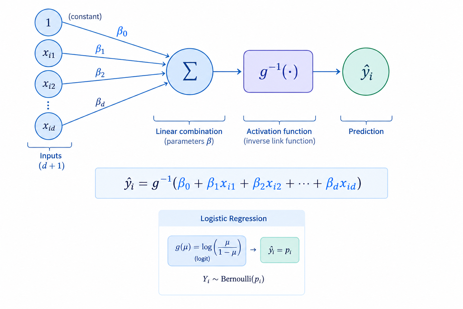
  • Logit link function: \(g(p)=\ln\left(\frac{p}{1-p}\right)\) is chosen here.
  • Its inverse is the well-known sigmoid function \(\sigma(x)=\frac{1}{1+e^{-x}}\).

Binary Target: Logistic Regression (cont.)

  • In summary if \(y_i\in\{0,1\}\) then the GLM model is \({\color{red}{\widehat{y}_i}}=g^{-1}(\text{x}_i^T{\color{blue}{\beta}})\), where \(g^{-1}({\color{blue}{z}})=\sigma(\color{blue}{z})=\frac{1}{1+e^{-\color{blue}{z}}}.\)
Binary Target: Logistic Regression Loss

  • For a binary response, \(y_i\sim{\cal B}({\color{red}{\widehat{y}_i}})\) with \({\color{red}{\widehat{y}_i}}=\sigma(\text{x}_i^T{\color{blue}{\beta}})\).
  • Likelihood on data \(D=\{(\text{x}_1,y_1),\dots,(\text{x}_n,y_n)\}\): \[\begin{align*}L({\color{blue}{\beta}})&=\prod_{i=1}^n\mathbb{P}(Y=y_i)\quad \text{with }P(Y=y_i)={\color{red}{\widehat{y}_i}}^{y_i}(1-{\color{red}{\widehat{y}_i}})^{1-y_i}\\ &=\prod_{i=1}^n{\color{red}{\widehat{y}_i}}^{y_i}(1-{\color{red}{\widehat{y}_i}})^{1-y_i}\quad(\text{with the convention: }0^0=1)\end{align*}\]
  • Log-likelihood: \(\ell({\color{blue}{\beta}})=\sum_{i=1}^n[y_i\ln({\color{red}{\widehat{y}_i}})+(1-y_i)\ln(1-{\color{red}{\widehat{y}_i}})]\).
  • The best parameter \({\color{blue}{\widehat{\beta}^*}}\) is chosen by maximizing \(\ell({\color{blue}{\beta}})\).
  • This is equivalent to ML framework: choose the best \({\color{blue}{\widehat{\beta}^*}}\) by mimimizing \(\text{Binary Cross-Entropy}({\color{blue}{\beta}})=-\ell({\color{blue}{\beta}}).\)

Binary Target: Coef. \({\color{blue}{\beta}}\) Interpretation

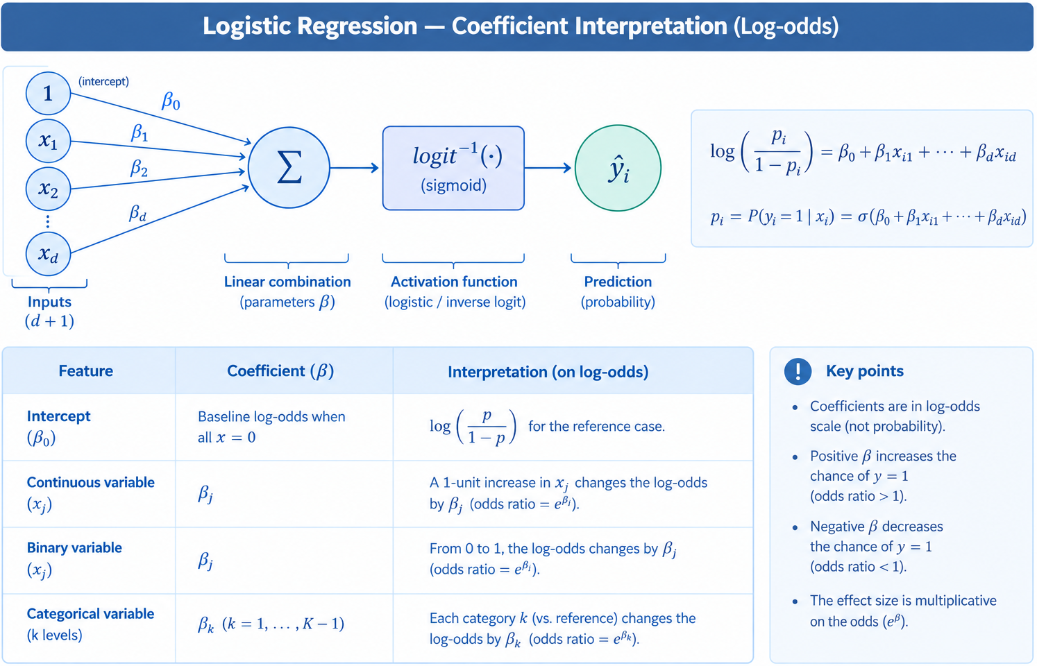
  • In binary classification, \(\color{blue}{\textbf{odds ratio}}=\frac{\mathbb{P}(y_i=1\mid X=\text{x}_i)}{\mathbb{P}(y_i=0\mid X=\text{x}_i)}=\frac{p_i}{1-p_i}\).
2.2 Example: Exam Passing

  • Suppose we model whether a student passes an exam: \[\log\left(\frac{p}{1-p}\right)= {\color{blue}{\beta_0}} + {\color{blue}{\beta_1}}\text{StudyHours}+{\color{blue}{\beta_2}}\text{Attendance}\]

  • If \({\color{blue}{\beta_1}} = 0.50\) then

    • Log-odds: A 1-hour increase in study time increases the log-odds of passing by \(\boxed{0.50}\), holding Attendance constant.
    • Odds ratio: Convert the coefficient to an odds ratio: \(e^{0.50}\approx 1.65\), meaning that 1-hour increase in study time multiplies the odds of passing by 1.65.
    • Percentage interpretation: \((1.65-1)\times100\%\approx65\%\) → The odds of passing increase by \(\approx\) 65% for each additional hour of study.
  • Important: This is a 65% increase in odds, not a 65%-point increase in probability.

3 Poisson Regression

3.1 Count Target

Poisson regression is suitable when the target is integer counts.

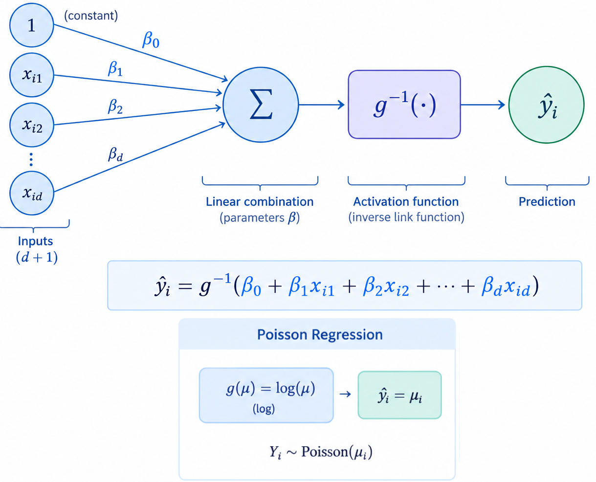
  • \(y_i\sim{\cal P}({\color{blue}{\lambda_i}})\), with \({\color{blue}{\lambda_i}}>0\).
  • What activation (inverse link) to use?
  • Step 1: Compute expectation \({\color{blue}{\lambda_i}}=\mathbb{E}[y_i\mid X=\text{x}_i]>0\)
  • Step 2: Which \(g:(0,\infty)\to\mathbb{R}\)? \(g(\lambda)=\ln({\lambda})\).
  • Step 3: Activation: \(g^{-1}({\color{blue}{z}})=e^{\color{blue}{z}}\).
  • Model: \(\boxed{{\color{red}{\widehat{y_i}}}=e^{\text{x}_i^T{\color{blue}{\beta}}}=e^{{\color{blue}{\beta_0}}+{\color{blue}{\beta_1}}\text{x}_{i1}+\cdots++{\color{blue}{\beta_d}}\text{x}_{id}}.}\)
  • Dission: How to estimate \({\color{blue}{\beta}}\)?
Poisson Coefficient Interpretation

  • In Poisson regression: \(\ln({\color{red}{\widehat{y}_i}})=\text{x}_i^T{\color{blue}{\beta}}={\color{blue}{\beta_0}}+{\color{blue}{\beta_1}}\text{x}_{i1}+\cdots++{\color{blue}{\beta_d}}\text{x}_{id}\).
  • Interpretation of coefficients: \(\boxed{e^{\color{blue}{\beta_j}}=\text{Multiplicative change in expected count}.}\)
  • For example, \({\color{blue}{\beta_j}}=0.10\) implies \(e^{0.10}\approx1.105.\) meaning a 1-unit increase in \(\text{X}_j\) is associated with approximately a 10.5% multiplicative increase in expected count, holding other variables constant.
  • Predictions:
    • Raw prediction: \({\color{red}{\widehat{y}_i}}=e^{\text{x}_i^T{\color{blue}{\widehat{\beta}^*}}}\).
    • Rounded prediction: \(\text{round}({\color{red}{\widehat{y}_i}})\).

Model Diagnostics

  • Poisson Deviance & Pearson Statistics are common criteria for assessing the goodness-of-fit of the model: \[\color{blue}{D}=2\sum_{i=1}^n\left[y_i\log\left(\frac{y_i}{\widehat{y}_i}\right)-(y_i-\widehat{y}_i)\right],\text{ and}\quad \color{red}{X^2}=\sum_{i=1}^n\frac{(y_i-{\color{red}{\widehat{y}_i}})^2}{{\color{red}{\widehat{y}_i}}}\]
    • \(\color{blue}{D}\) and \(\color{red}{X^2}\approx\text{DOF}=n-d-1\) indicates good fit.
  • Dispearsion for checking dispersion of predictions: \[\text{Dispersion }{\color{red}{\widehat{\phi}}}=\frac{\color{red}{X^2}}{n-d-1}\]
    • \({\color{red}{\widehat{\phi}}}<1\): Underdispersed predictions compared to actual data.
    • \({\color{red}{\widehat{\phi}}}>1\): Overdispersed predictions compared to actual data.

For more criteria, read STAT 462 notes.

Summary

Comparison

Linear Logistic Poisson
Target Continuous Binary Count
Distribution Gaussian Bernoulli Poisson
Mean \(\mu\) \(p\) \(\lambda\)
Linear predictor \(X{\color{blue}{\beta}}\) \(X{\color{blue}{\beta}}\) \(X{\color{blue}{\beta}}\)
Link Identity Logit Log
Inverse link \(\color{blue}{z}\) \(\sigma({\color{blue}{z}})\) \(e^\color{blue}{z}\)
Loss MSE Binary CE Poisson NLL
Coefficient interpretation Additive Odds ratio Multiplicative

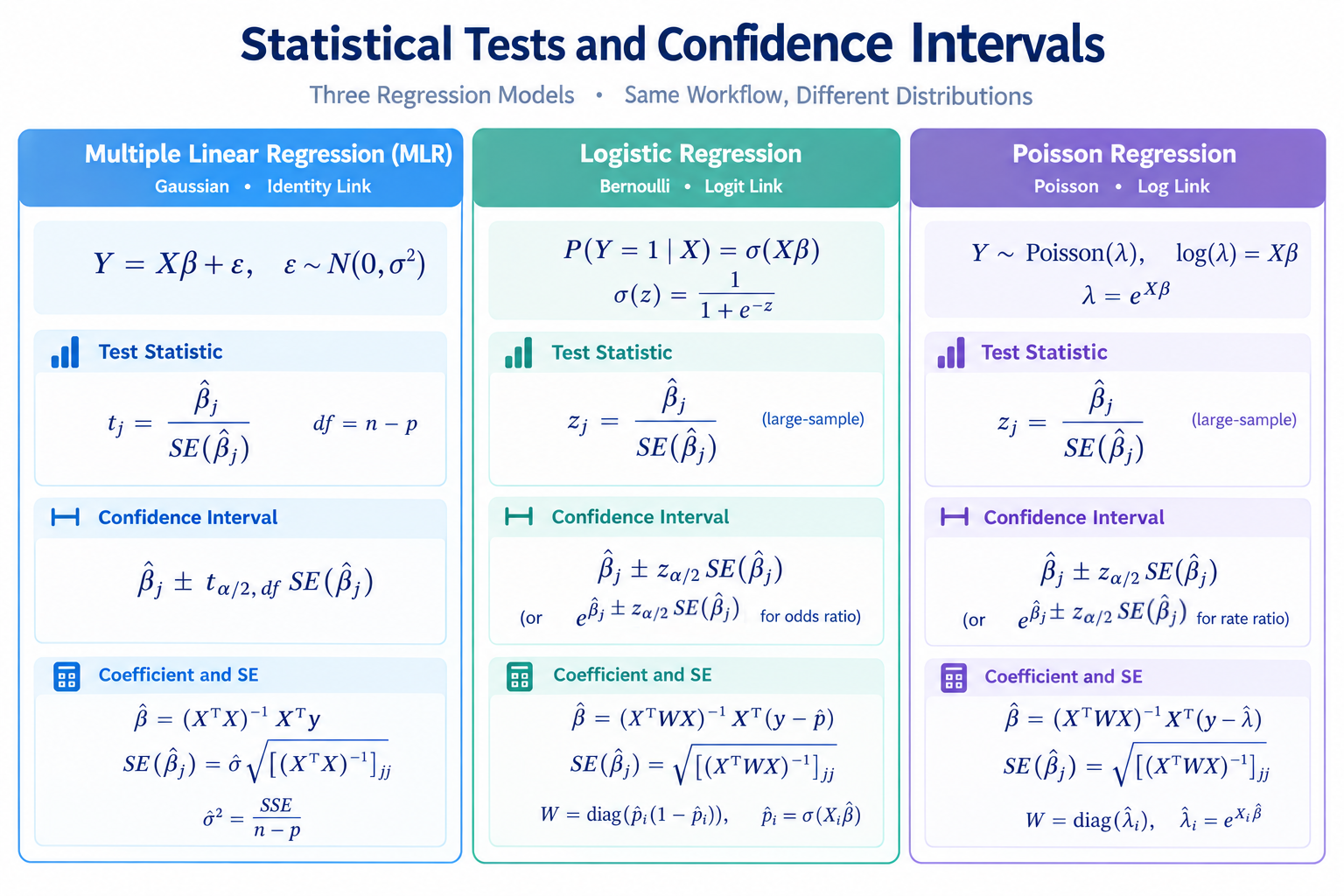
4 Statistical Test & CIs

4.1 Significance of coefs & CIs

Diagnostics: What Else to Check?

  • Diagnostics is also required when we move from LR to GLMs.
  • 1. Is the model appropriate?
    • Is the response distribution reasonable?
  • 2. Are important predictors missing?
    • Use DA to detect useful variables,
    • Nonlinear effects (feature engineering),
    • Interactions (mixture of variables).
  • 3. Are there problematic observations?
    • Outliers,
    • High-leverage observations,
    • Influential observations.

4.4 GLM Summary

  • The entire GLM framework can be summarized as \[\boxed{X\longrightarrow X\beta\longrightarrow g^{-1}(X{\color{blue}{\beta}})\longrightarrow\mu=E[Y\mid X].}\]

  • Main types: \[\boxed{\begin{aligned}\text{Continuous}&\rightarrow\text{Linear Regression}\\\text{Binary}&\rightarrow\text{Logistic Regression}\\\text{Count}&\rightarrow\text{Poisson Regression}\end{aligned}}\]

  • The parameter \(\color{blue}{\beta}\) is estimated using MLE that leads to different types of loss function in ML.

🥳 Yeahhhh 🥂!!!


Let’s take a break!

Appendix 1

  • The Poisson model \(y_i\sim{\cal P}({\color{red}{\widehat{y_i}}})\) with \({\color{red}{\widehat{y_i}}}=e^{\text{x}_i^T{\color{blue}{\beta}}}\). The Poisson PMF: \[P(Y=y_i)=\frac{e^{-{\color{red}{\widehat{y_i}}}}{{\color{red}{\widehat{y_i}}}}^{y_i}}{y_i!}.\]

  • Log-likelihood: \(\ell({\color{blue}{\beta}})=\sum_i\left[-\log(y_i!)-{\color{red}{\widehat{y_i}}}+y_i\log({\color{red}{\widehat{y_i}}})\right].\)

  • Using \(\log({\color{red}{\widehat{y_i}}})=\text{x}_i^T{\color{blue}{\beta}}\) one has the negative log-likelihood, ignoring constants, becomes \(\boxed{\text{Poisson loss}({\color{blue}{\beta}})=\sum_{i=1}^n\left[e^{\text{x}_i^T{\color{blue}{\beta}}}-y_i\text{x}_i^T{\color{blue}{\beta}}\right].}\)

  • One can learn the best parameters \({\color{blue}{\beta}}\) by minimizing \(\text{Poisson loss}\).