Bayesian Inference


INS-605: Data Analysis II

Lecturer: Dr. Sothea HAS

helpful resources

🌐 Understading the Difference between Bayesian and Frequentist Statistics by Fornacon-Wood et al. (2021).

Learning Objectives

By the end of this lecture, students should be able to:

  • Explain the motivation for Bayesian inference.
  • Distinguish Frequentist and Bayesian interpretations.
  • Apply Bayes’ theorem to estimate parameters.
  • Explain the roles of the prior, likelihood, and posterior.
  • Interpret Bayesian credible intervals.
  • Perform Bayesian updating using a Beta-Binomial model.
  • Understand posterior predictive inference.

1 Motivation

1.1 Frequentist Inference

  • Frequentist framework:
    • The parameter is fixed.
    • The parameter is unknown.
    • The data are random.
  • Example: Eggs survival model: \(X_1,\ldots,X_n \sim \mathcal{B}(\color{red}{p})\), \(\color{red}{p}\) is unknown.
  • Frequentist inference:
    • Point estimate: find \(\color{red}{\hat{p}}\), for example by maximizing the likelihood function.
  • Interval estimate: find an interval \(I_{\color{green}{1-\alpha}}=[a(\color{red}{\hat{p}}), b(\color{red}{\hat{p}})]\) with \(\mathbb{P}(\color{red}{p}\in I_{\color{green}{1-\alpha}})=\color{green}{1-\alpha}\).

Frequentist

The parameter is fixed and unknown. The fish doesn't move — we just observe what surfaces.

surface = observed data
fixed parameter
x₁
x₂
x₃
x₄
x₅

Position: a single fixed value, and the uncertainty is due to the bubbles rising.

1.2 Bayesian Thinking

  • The parameter is uncertain & data is uncertain but observed.
  • Ex: Before observing the data, you may belive that it’s fair (\(p=0.5\)). However, after some tosses, you may change your belief about the parameter \(p\).
Bayesian

The parameter itself has a distribution. The fish swims and leaves its own trail of data behind.

surface = observed data
x₁
x₂
x₃
x₄
x₅
x₆

Position: The fish itself is moving and can be anywhere, governs by the density function.

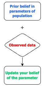
  • Prior: Your initial belief in value of parameter.
  • Bubbles: Data \(X_1,X_2,...\) are observed.
  • Posterior: Your updated belief in value of parameter after observing the data.

Frequentist vs Bayesian

Question Frequentist Bayesian
What is the parameter? Unknown and fixed Unknown and uncertain
What is random? Data Parameter uncertainty \(\to\) data
Main tool Likelihood Bayes’ theorem
Main result Point estimate (MLE) Posterior distribution
Interval Confidence interval Credible interval
Prediction Based on estimated parameters Based on posterior uncertainty

2 Bayes’ Theorem

2.1 Bayes’ Theorem for Events

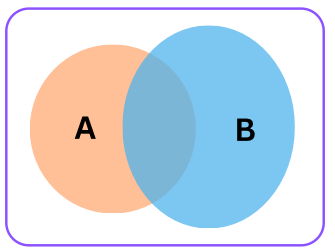
  • For two events \(A\) and \(B\) with non-zero probabilities, Bayes’ theorem states:

\[P(A\mid B)=\frac{P(B\mid A)P(A)}{P(B)}\]

where:

  • \(P(A)\): prior probability
  • \(P(B\mid A)\): likelihood
  • \(P(B)\): evidence
  • \(P(A\mid B)\): posterior probability

Example: Disease Testing

  • Suppose a disease affects 50% of the population (\(\color{blue}{D=1}\)).
  • A test is 99% accurate:
    • Correctly identifies 99% of those with the disease,
    • Correctly identifies 99% of those without the disease.
  • If a person tests positive, how likely do you think they actually have the disease?

\[P(\color{blue}{D=1}\mid \color{red}{T=1}) = \frac{P(\color{red}{T=1}\mid \color{blue}{D=1})P(\color{blue}{\color{blue}{D=1}})}{P(\color{red}{T=1})}.\]

  • \(P(\color{red}{T=1}\mid \color{blue}{D=1}) = 0.99\).
  • \(P(\color{blue}{D=1}) = 0.5\).
  • Testing positive:
    \(\begin{align*}& P(\color{red}{T=1})\\ = &\ 0.99\times0.5 + 0.01\times0.5\\ = &\ 0.5 \text{ (why?)}\end{align*}\)
  • Hence, \(P(\color{blue}{D=1}\mid \color{red}{T=1}) = 0.99\).
  • Is this surprising?

Example: Rare Disease Testing

  • Suppose a disease affects only 1% of the population.
  • \(P(\color{red}{T=1}\mid \color{blue}{D=1}) = 0.99\).
  • \(P(\color{blue}{D=1}) = 0.01\).
  • Testing positive:
    \(\begin{align*}& P(\color{red}{T=1})\\ = &\ 0.99\times0.01 + 0.01\times0.99\\ = &\ 0.0198 \text{ (why?)}\end{align*}\)
  • Hence, \(P(\color{blue}{D=1}\mid \color{red}{T=1}) = \frac{0.99\times0.01}{0.0198} = 0.5.\)
  • Is this surprising?
  • If there are 1M people, then
Test Sick Healthy
Positive 9,900 9,900
Negative 100 980,100
Total 10,000 1,000,000
  • For very rare diseases, even a highly accurate test can produce a large number of false positives (9,900).
  • A second test can help reduce false positives.

2.2 Bayes’ Theorem for Parameters

  • Let \(\color{blue}{x}\) be the observed data and \(\color{red}{\theta}\) be an unknown parameter.

\[\underbrace{p(\color{red}{\theta}\mid \color{blue}{x})}_{\text{Posterior}}=\frac{\overbrace{p(\color{blue}{x}\mid\color{red}{\theta})}^{\text{Likeihood}}\overbrace{p(\color{red}{\theta})}^{\text{Prior}}}{\underbrace{p(\color{blue}{x})}_{\text{How likely to observe data }\color{blue}{x}}}\propto p(\color{blue}{x}\mid\color{red}{\theta})p(\color{red}{\theta}).\]

  • Coin toss example, let \(\color{red}{\theta=p}\) be unknown probability of head per toss (success).
    • Prior: \(\color{red}{\theta}\sim\color{purple}{\operatorname{Beta}(2,2)}\), i.e., \(f(\color{red}{\theta})=\frac{\color{red}{\theta}(1-\color{red}{\theta})}{B(2,2)}\).
    • Data: \(N=30\) and \(n(H)=\color{green}{18}\).
    • Likelihood: \(p(\color{blue}{x}=\color{green}{18}\mid \color{red}{\theta})=\binom{30}{\color{green}{18}}\color{red}{\theta}^{\color{green}{18}}(1-\color{red}{\theta})^{12}\).

Read more about Beta distribution on Wikipedia.

2.2 Bayes’ Theorem for Parameters

  • Let \(\color{blue}{x}\) be the observed data and \(\color{red}{\theta}\) be an unknown parameter.

\[\underbrace{p(\color{red}{\theta}\mid \color{blue}{x})}_{\text{Posterior}}=\frac{\overbrace{p(\color{blue}{x}\mid\color{red}{\theta})}^{\text{Likeihood}}\overbrace{p(\color{red}{\theta})}^{\text{Prior}}}{\underbrace{p(\color{blue}{x})}_{\text{How likely to observe data }\color{blue}{x}}}\propto p(\color{blue}{x}\mid\color{red}{\theta})p(\color{red}{\theta}).\]

\[\begin{align*}p(\color{red}{\theta}\mid \color{blue}{x}=\color{green}{18})&\propto p(\color{blue}{x}=\color{green}{18}\mid\color{red}{\theta})p(\color{red}{\theta})\\ &= \left[\binom{30}{\color{green}{18}}\color{red}{\theta}^{\color{green}{18}}(1-\color{red}{\theta})^{12}\right][\color{red}{\theta}(1-\color{red}{\theta})]\\ &\propto \color{red}{\theta}^{19}(1-\color{red}{\theta})^{13}\\ &=\color{red}{\theta}^{\color{purple}{20}-1}(1-\color{red}{\theta})^{\color{purple}{14}-1}\\ \Rightarrow \underbrace{(\color{red}{\theta}\mid \color{blue}{x}=\color{green}{18})}_{\text{New belief of }\color{red}{\theta}}&\sim\color{purple}{\text{Beta}(\color{purple}{20},\color{purple}{14})}\quad (\color{purple}{\text{Posterior}}).\end{align*}\]

Influence of Prior

  • Prior belief is expressed by \(p(\color{red}{\theta})\) (dashed lines), and when observing data \(\color{blue}{x}\), it updates to a new belief (posterior) \(p(\color{red}{\theta}\mid \color{blue}{x})\).
  • Different priors can result in different posterior distributions.

Weak and Informative Priors

  • A prior can be:
    • Weakly or strongly informative.
    • Symmetric or asymmetric.
    • Based on previous studies or expert knowledge.
    • Chosen for mathematical convenience.
  • For example: \(\color{red}{\theta}\sim\color{blue}{\operatorname{Beta}(1,1)}\) is uniform on \(\color{blue}{U[0,1]}\).
  • Meanwhile: \(\color{red}{\theta}\sim\color{orange}{\operatorname{Beta}(20,5)}\) expresses a stronger belief that \(\color{red}{\theta}\) is relatively large.

Python: Visualizing Beta Priors

3 Posterior Mean

3.1 Posterior Mean

  • In Bayesian Framework, Posterior Mean, the expected value of the parameter given the observed data, i.e., \(\mathbb{E}[\color{red}{\theta}|\color{blue}{x}]\), is a point summary of the parameter of the population.
  • After computing the posterior, we compute its expectation.
    • For example if \((\color{red}{\theta}|\color{blue}{x})\sim\text{Beta}(\alpha, \beta)\Rightarrow \mathbb{E}[\color{red}{\theta}|\color{blue}{x}]=\frac{\alpha}{\alpha+\beta}\).

3.2 MLE vs Posterior Mean

  • Let’s compare MLE and Posterior Mean on Coin Toss example.
  • Maximum Likelihood Estimator (MLE):
    • Log-likelihood: \(\ell(\color{red}{\theta})=18\ln(\color{red}{\theta})+12\ln(1-\color{red}{\theta})+\text{cont.}\)
    • \(\ell'(\color{red}{\theta})=18/\color{red}{\theta}-12/(1-\color{red}{\theta})\)
    • MLE: \(\color{red}{\widehat{\theta}}=18/30=0.6.\)
    • This is purely data-driven.
  • Posterior Mean:
    • For prior \(\color{red}{\theta}\sim \text{Beta}(2,2)\)
    • Posterior \((\color{red}{\theta}\mid \color{blue}{x})\sim \text{Beta}(20,14)\)
    • Posterior Mean: \(\color{green}{\widehat{\theta}}=\mathbb{E}(\color{red}{\theta}\mid \color{blue}{x})=\frac{\alpha}{\alpha+\beta}=\frac{20}{20+14}=0.5882.\)

4 Credible Intervals

4.1 Credible Intervals

  • Posterior mean is point summary of the parameter.
  • A credible interval is an interval estimate of a parameter that captures the uncertainty in the parameter.
  • If \(\color{red}{\alpha}\in (0,1)\), be a level of error, then a credible interval at level \(1-\color{red}{\alpha}\) of \(\color{red}{\theta}\) denoted by \(\text{CI}_{1-\color{red}{\alpha}}=[a,b]\) such that \(\mathbb{P}(a\leq \color{red}{\theta}\leq b\mid \color{blue}{x})=1-\color{red}{\alpha}\).
  • This means:

Given the observed data \(\color{blue}{x}\) and the prior \(p(\color{red}{\theta})\), there is a \(1-\color{red}{\alpha}\) posterior probability that \(\color{red}{\theta}\in[a,b]\).

  • The interval is calculated from the posterior distribution.

Credible Interval for Coin Toss

Bayesian Prediction

  • Bayesian inference can also predict a future observation.
  • Suppose we want to predict the chance of getting head next:

\[\begin{align*}p(X_{new}=1\mid \color{blue}{x})&=\int_{0}^1\underbrace{p(X_{new}=1\mid \color{red}{\theta})}_{\text{Chance of head}}p(\color{red}{\theta}\mid \color{blue}{x})d\color{red}{\theta}\\ &=\int_{0}^1\color{red}{\theta}p(\color{red}{\theta}\mid \color{blue}{x})d\color{red}{\theta}\\ &=\mathbb{E}(\color{red}{\theta}\mid \color{blue}{x})=20/34=\color{green}{0.5882}.\end{align*}\]

  • Remark Bayesian theory fits well with online learning as Posterior can be considered a new Prior for the next observation.

Frequentist vs Bayesian Workflow

  • Frequentist:
Choose probability model

Construct likelihood

Optimize likelihood

Obtain MLE

Construct confidence interval

Make predictions
  • Bayesian:
Choose probability model

Specify prior distribution

Construct likelihood

Combine prior and likelihood

Obtain posterior distribution

Calculate posterior summaries

Construct credible intervals

Make posterior predictions

Conjugate Priors

Likelihood Prior Posterior
Bernoulli/Binomial Beta Beta
Poisson Gamma Gamma
Normal mean with known variance Normal Normal
Multinomial Dirichlet Dirichlet
  • Conjugacy makes Bayesian inference mathematically convenient.
  • Many real-world models do not have a closed-form posterior.
    • Logistic regression
    • Neural network models…

5 Bootstrap

5.1 What is Bootstrap?

  • We have only one dataset: \[D = \{x_1,x_2,\ldots,x_n\}\]
  • But we want to know:
    • How variable is our estimator?
    • What would happen with another sample?
    • How confident are we in our estimate?
  • It allows us to estimate the sampling distribution of an estimator.
  • It is a key tool for many ML models: RF, Boosting, etc.

Bootstrap idea

  • Treat the observed data as an approximation of the population and repeatedly resample with replacement.

  • Each bootstrap sample \(D_j^*\to\) an estimator \(\widehat{\theta}_j\).
  • The uncertainty of \(\widehat{\theta}\) is quantified by \(\text{SE}(\widehat{\theta})\).

95% Bootstrap Confidence Interval

  • By sorting all bootstrap estimates, we can find the 95% confidence interval (CI) as the middle range \([q_{0.025},q_{0.975}]\) of the estimates:

\[ \boxed{ CI_{95\%} = [q_{0.025},q_{0.975}] } \]

Key idea:

Bootstrap approximates the sampling distribution without repeatedly collecting new datasets.

From Bootstrap to Bagging

  • Bootstrap is also useful for machine learning models.
  • Train a model on each bootstrap dataset: \[f_1(x),f_2(x),\ldots,f_B(x)\]
  • Then average their predictions: \[\boxed{\hat f_{\text{bag}}(x)=\frac{1}{B}\sum_{b=1}^{B}f_b(x)}\]
  • This is called: Bootstrap AggregatingBagging.

Bagging in Practice

What does it aim to do?

  • Individual models can have high variance and very biased.
  • Averaging several models can make the final prediction more stable (reducing variance).
  • Example:
    • A decision tree built on a bootstrap sample → high variance
    • Many bootstrap samples → many high varianced trees
    • Average predictions → more stable prediction (Bagging / Random Forest).

4. Why Does Averaging Reduce Variance?

  • Suppose every model has prediction variance: \[\mathbb{V}(f_b)=\sigma^2\]

  • If models were independent: \[\mathbb{V}\left(\frac{1}{B}\sum_{b=1}^{B}f_b\right)=\frac{\sigma^2}{B}\]

  • Therefore: \(\boxed{B\uparrow\quad\Rightarrow\quad \text{Variance}\downarrow}\)

Visualization of Random Forest

But bootstrap models are correlated!

  • They are trained on overlapping samples.
  • If pairwise correlation is \(\rho\): \(\boxed{\mathbb{V}(\bar f)=\sigma^2\left[\rho+\frac{1-\rho}{B}\right]}\).
  • As \(B\) gets large: \(\mathbb{V}(\bar f)\rightarrow\rho\sigma^2\).
  • Important ML insight:

More models reduce variance, but correlation creates a variance floor.

Summary

  • Bootstrap helps estimate:
    • Standard errors
    • Confidence intervals
    • Sampling distributions
    • Uncertainty of statistics
    • Variance reduction in ML models…

🥳 Yeahhhh 🥂!!!


Let’s take a break!