Probability & Simulation

INS-605: Data Analysis II

Lecturer: Dr. Sothea HAS

Content

• 1 Introduction & Motivation
• 2 Probability Distributions & Models
• 3 Parameter Estimation
• 4 Simulation Methods

helpful resources

🌐 Introduction to Probability for Data Science, Stanley Chan.

1 Introduction & Motivation

1.1 History

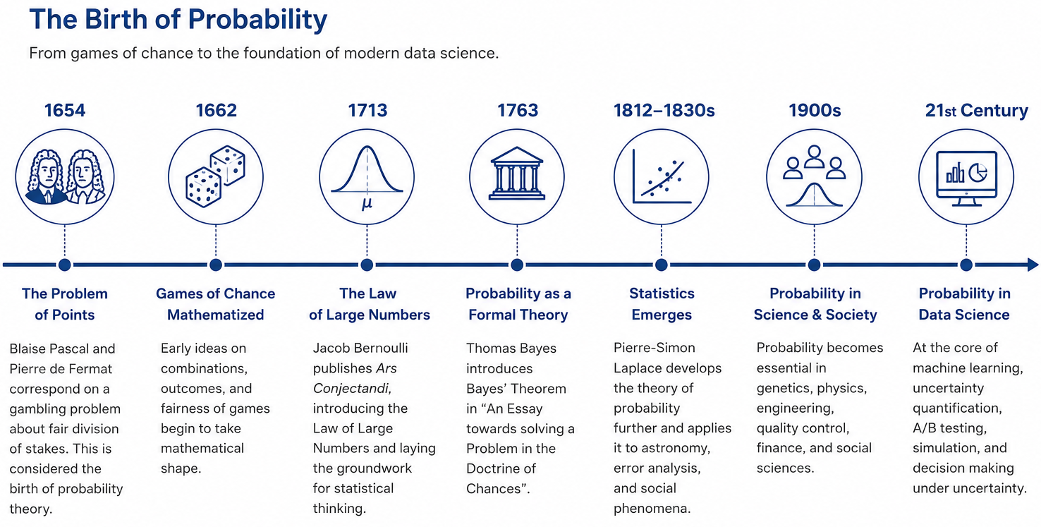
• Our focus: Probability in Data Science & Simulation.

1.2 Probability in Data Science

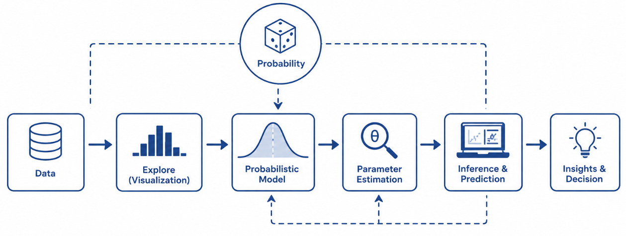
• In Data Science, probability is important in various parts:
  • Sampling & Data Collection: Gathering unbiased, representative data.
  • Anomaly Detection: Spotting rare events and unexpected outliers.
  • Hypothesis Testing: Proving whether observed patterns are real or random chance.
  • Unsupervised Clustering: Grouping similar data based on density and likelihood.
  • Predictive & Generative Models: Forecasting outcomes and synthesizing new data.

1.3 Motivation

• Signal vs. Noise: Real-world data seamlessly blends meaningful patterns with inherent uncertainty.
• Avoid Misleading Insights: To extract useful signal , we must quantify noisy components .
• Characterize Uncertainty: The first step toward reliable analysis is understanding how uncertainty behaves.
• Role of Probability: Probability theory serves as a foundational tool to quantify and manage this randomness.

import plotly.express as px
import plotly.graph_objects as go 
import pandas as pd
from plotly.subplots import make_subplots

data = pd.read_csv(path_baby)
fig = make_subplots(
    rows=1,
    cols=4,
    specs=[
        [
            {"type": "Histogram"},
            {"type": "Bar"},
            {"type": "Histogram"},
            {"type": "Histogram"}
        ]
    ],
    subplot_titles=[
        'Age of Mother', 
        'Father Race',
        'Total Pregnancies',
        'Birth Weight (kg)'
        ],
    horizontal_spacing=0.1
)

fig.add_trace(
    go.Histogram(
        x=data.MAGE,
        hovertemplate="Age: %{x}<br>Count: %{y}",
        showlegend=False
    ),
    row=1,
    col=1
)
fig.update_yaxes(
    row=1,
    col=1,
    title='Count'
)
mean_age = data.MAGE.mean()
fig.add_trace(
    go.Scatter(
        x=[mean_age] * 2,
        y=[0, 6000],
        mode='lines',
        line = dict(
            width=3,
            color='red',
            dash='dash'
        ),
        hovertext=f'Mean: {mean_age}',
        showlegend=False
    ),
    row=1,
    col=1
)
racedad = data.RACEDAD.value_counts()
fig.add_trace(
    go.Bar(
        x=racedad.index,
        y=racedad.values,
        hovertemplate="Race: %{x}<br>Proportion: %{y}",
        showlegend=False
    ),
    row=1,
    col=2
)
fig.update_yaxes(
    title='Count (log scaled)',
    type='log',
    row=1,
    col=2
)
fig.add_trace(
    go.Histogram(
        x=data.TOTALP,
        hovertemplate="Age: %{x}<br>Count: %{y}",
        showlegend=False
    ),
    row=1,
    col=3
)
mean_tot = data.TOTALP.mean()
fig.add_trace(
    go.Scatter(
        x=[mean_tot] * 2,
        y=[0, 35000],
        mode='lines',
        line = dict(
            width=3,
            color='red',
            dash='dash'
        ),
        hovertext=f'Mean: {mean_tot}',
        showlegend=False
    ),
    row=1,
    col=3
)
fig.update_yaxes(
    title='Count',
    row=1,
    col=3
)
RATE = 0.453592
fig.add_trace(
    go.Histogram(
        x=data.BWEIGHT * RATE,
        hovertemplate="Weight: %{x}<br>Count: %{y}",
        showlegend=False
    ),
    row=1,
    col=4
)
mean_w = data.BWEIGHT.mean() * RATE
fig.add_trace(
    go.Scatter(
        x=[mean_w] * 2,
        y=[0, 2500],
        mode='lines',
        line = dict(
            width=3,
            color='red',
            dash='dash'
        ),
        showlegend=False
    ),
    row=1,
    col=4
)
fig.update_yaxes(
    title='Count',
    row=1,
    col=4
)
fig.update_layout(
    width=950,
    height=200,
    title="Some Variables from <a href='https://www.kaggle.com/datasets/ashiskb/baby-birthweight-dataset?select=baby-weights-dataset.csv'>Baby Weight Dataset</a> " + str(data.shape),
    margin=dict(
        t=50,
        l=10,
        r=10,
        b=10
    )
)

2 Probability Distributions & Models

2.1 Discrete Random Variables

Review

• To describe data mathematically, we use Random Variables denoted by \(X,Y,Z,\dots\).
• Unlike data type, we classify RV into two different types:
  • Discrete V.R., \(X\in\mathcal{S}\subset \mathbb{N}=\{1,2,3,...\}\) (\(\mathcal{S}\): sample space.)
  • Continuous V.R., \(X\in\mathcal{S}\in\mathbb{R}\).

fig_race = go.Figure()
fig_race.add_trace(
    go.Bar(
        x=racedad.index,
        y=racedad.values,
        text=racedad.values,
        hovertemplate="Race: %{x}<br>Proportion: %{y}",
        showlegend=False
    )
)
fig_race.update_yaxes(
    title='Count (log scaled)',
    type='log'
)
fig_race.update_layout(
    width=400,
    height=170,
    title='Father Race'
).show()

• If \(X\): Race of Father,
  • \(\mathcal{S}=\{0,1,\dots,9\}\).
• If a father is chosen at random, how likely that his race is ‘4’?

Probability Mass Function (PMF)

• If \(Y\): Number of Pregnancies,
  • \(\mathcal{S}_Y=\{1,2,3,\dots\}\)
  • \(\hat{\mathbb{P}}(Y=4)\approx\frac{9624}{101400}=\) 0.09.

	proportion
TOTALP
1	0.330355
2	0.301440
3	0.189458
4	0.094911
5	0.044546
6	0.020414
7	0.009536
8	0.004517
9	0.002209
10	0.001183

	proportion
TOTALP
11	0.000700
12	0.000394
13	0.000128
14	0.000069
17	0.000039
15	0.000039
18	0.000020
16	0.000020
20	0.000010
19	0.000010

fig_preg = go.Figure()
fig_preg.add_trace(
    go.Histogram(
        x=data.TOTALP,
        text=data.TOTALP.value_counts(),
        hovertemplate="Total Pregnancies: %{x}<br>Count: %{y}",
        showlegend=False,
        marker=dict(
            color = "#8AE4F2",
            line=dict(
                color='white',
                width=1
            )
        )
    )
)
fig_preg.add_trace(
    go.Scatter(
        x=[mean_tot] * 2,
        y=[2000, 33500],
        mode='lines',
        name=r'$\color{blue}{\mu_X}$',
        line = dict(
            width=3,
            color='blue',
            dash='dash'
        ),
        hovertext=f'Mean: {round(mean_tot,2)}',
        visible='legendonly'
    )
)
fig_preg.update_yaxes(
    title='Count'
)
fig_preg.update_layout(
    width=450,
    height=200,
    title='Total Pregnancies'
).show()

• Probability Mass Function \(f\): \[f(x_i)=p_i=\mathbb{P}(X=x_i), \forall x_i\in\mathcal{S}\]
• It describes how likely each possible outcome \(x_i\) is in a random experiment involving \(X\).
• Roughly: We can approximate usual or unlikely outcomes and other characteristics of \(X\).

Numerical Summary of RV

• Expectation of a DRV \(X\) is the mean/average over the outcomes \(x_i\)’s weighted by their corresponding chances \(p_i\)’s, .i.e., \[\color{blue}{\mu_X}=\mathbb{E}(X)=\sum_{i\geq 1}x_ip_i=x_1p_1+x_2p_2+\dots\]
  • Note: Mean/average of real data is realized with \(p_i=\hat{p}_i=\frac{n_i}{n}.\)
  • Ex: Total Pregnancies, \(\overline{X}_n\) = 2.38.

---

• Variance of a DRV \(X\) is the average squared gaps between outcomes \(x_i\)’s and the mean \(\color{blue}{\mu_X}\) weighted by \(p_i\)’s, .i.e., \[\color{red}{\sigma_X^2}=\color{red}{\mathbb{V}(X)}=\mathbb{E}[(X-\color{blue}{\mu_X})^2]=\sum_{i\geq 1}(x_i-\color{blue}{\mu_X})^2p_i.\]

fig_preg.show()

• Large variance indicates the wider dispersion of outcomes or more uncertainty of the RV
• Smaller variance indicates lesser uncertainty.
• Standard Deviation (SD) is more common to use as it is in the same units as the R.V: \(\color{red}{\sigma_X}=\sqrt{\color{red}{\mathbb{V}(X)}}\).

Some common DRVs

Bernoulli Distribution

• For binary data with only two possible outcomes {1 : ‘success’, 0 : ‘failure’}, the Bernoulli Distribution is used.
• Ex: Gender, Yes/No, Sick/Healthy, etc.
• Let \(X\in\mathcal{S}=\{\color{red}{0},\color{green}{1}\}\) be such a data, denoted by \(X \sim \mathcal{B}(\color{green}{p})\), where \(\color{green}{p}\) is the probability of success, i.e., \(\color{green}{p}=\mathbb{P}(X=\color{green}{1})\).
• PMF of \(X\) is given by: \(\mathbb{P}(X=\color{green}{1})=\color{green}{p}\ \text{and } \mathbb{P}(X=\color{red}{0})=\color{red}{1-p}=\color{red}{q}\).

\(X=k\)	\(\color{green}{1}\)	\(\color{red}{0}\)
\(\mathbb{P}(X=k)\)	\(\color{green}{p}\)	\(\color{red}{1-p}\)

• If \(X\sim{\cal B}(p)\), then
  • \(\mathbb{E}[X]=\color{green}{p}\)
  • \(\text{Var}(X)=\color{green}{p}\color{red}{(1-p)}\)
  • \(\text{SD}(X)=\sqrt{\color{green}{p}\color{red}{(1-p)}}\).

Some common DRVs (Cont.)

Binomial Distribution

• The Number of Total Sucesses occurs in a series of n independent Bernoulli trails yield a Binomial distribution, \(X\sim{\cal Bin}(n,\color{green}{p})\).
• Ex: The number of sick children in room of 25 newborns…
• If \(X\sim{\cal Bin}(n,\color{green}{p})\), then \(\mathcal{S}=\{0,1,..,n\}\) and its PMF is given by: \[P(X=\color{purple}{k})=\binom{n}{\color{purple}{k}}\color{green}{p}^{\color{purple}{k}}\color{red}{(1-p)}^{n-\color{purple}{k}} \text{ for } \color{purple}{k}=0,...,n.\]

\(X=k\)	\(0\)	\(1\)	\(2\)	\(\dots\)	\(n-1\)	\(n\)
\(\mathbb{P}(X=k)\)	\(\color{red}{(1-p)^n}\)	\(n\color{green}{p}\color{red}{(1-p)^{n-1}}\)	\(\frac{n(n-1)}{2!}\color{green}{p^2}\color{red}{(1-p)^{n-2}}\)	\(\dots\)	\(n\color{green}{p^{n-1}}\color{red}{(1-p)}\)	\(\color{green}{p^n}\)

• If \(X\sim{\cal Bin}(n,p)\), then
  • \(\mathbb{E}[X]=n\color{green}{p}\)
  • \(\text{Var}(X)=n\color{green}{p}\color{red}{(1-p)}\)
  • \(\text{SD}(X)=\sqrt{n\color{green}{p}\color{red}{(1-p)}}\).

Some common DRVs (Cont.)

Poison Distribution

• A Poison RV \(X\) counts the number of (rare) events in a fixed interval of time or space, \(X\sim{\cal P}(\color{red}{\lambda}), \color{red}{\lambda}>0\).
• Ex: Number of wrong money transfers in an app per day, or Number of Total Pregnancies a woman may have…
• If \(X\sim{\cal P}(\color{red}{\lambda})\), then \(\mathcal{S}=\{0,1,2,3,...\}\) and its PMF is given by: \[P(X=\color{purple}{k})=e^{-\color{red}{\lambda}}\frac{\color{red}{\lambda}^{\color{purple}{k}}}{\color{purple}{k}!} \text{ for } \color{purple}{k}=0,...,n.\]

\(X=k\)	\(0\)	\(1\)	\(2\)	\(3\)	\(4\)	\(\dots\)
\(\mathbb{P}(X=k)\)	\(e^{-\color{red}{\lambda}}\)	\(e^{-\color{red}{\lambda}}\color{red}{\lambda}\)	\(e^{-\color{red}{\lambda}}\frac{\color{red}{\lambda}^2}{2!}\)	\(e^{-\color{red}{\lambda}}\frac{\color{red}{\lambda}^3}{3!}\)	\(e^{-\color{red}{\lambda}}\frac{\color{red}{\lambda}^4}{4!}\)	\(\dots\)

• If \(X\sim{\cal Bin}(n,p)\), then
  • \(\mathbb{E}[X]=\text{Var}(X)=\color{red}{\lambda}\)
  • \(\text{SD}(X)=\sqrt{\color{red}{\lambda}}\).

Expectation, Variance & SD

Note

Theoretical Concepts

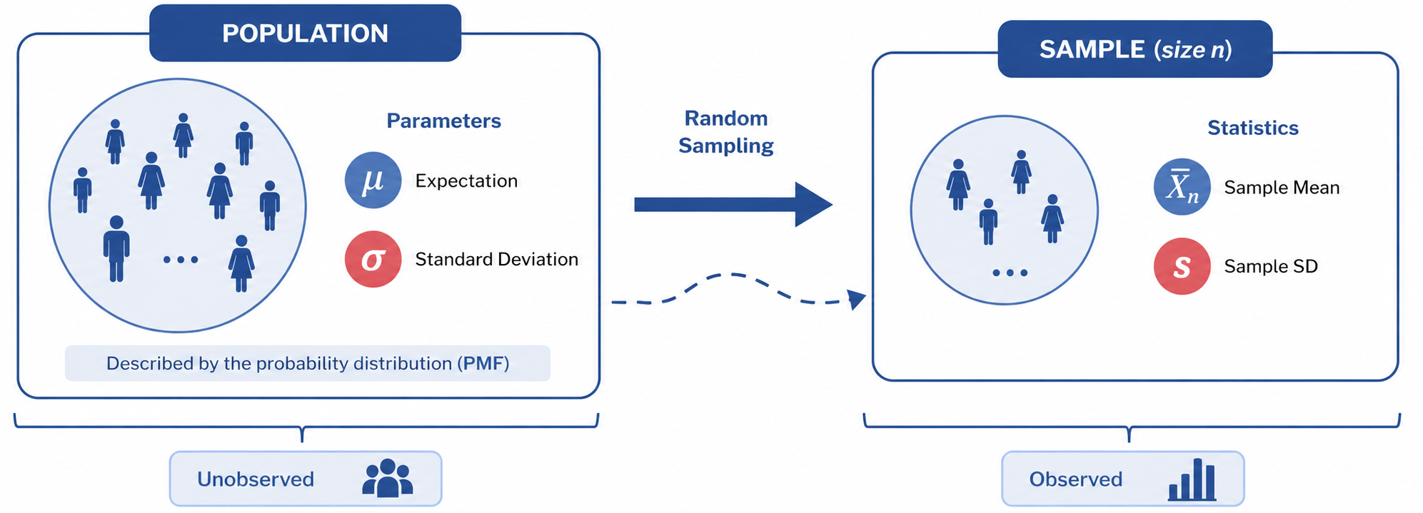
• Expectation: \(\color{blue}{\mu_X}=\sum_{i\geq 1} x_i p_i\).
• Variance: \(\color{red}{\sigma_X^2}=\sum_{i\geq 1} (x_i-\color{blue}{\mu_X})^2p_i\).
• SD: \(\color{red}{\sigma_X}=\sqrt{\color{red}{\sigma_X^2}}\).
• Theoretical concepts.
• Computed from a probability distribution (PMF).
• Never be computed from data.
• They are called parameters of the population.
• Example:
  • Your true weight/height.
  • True average birth weight in Cambodia.
  • Coefficient of Variation (\(\sigma/\mu\)) in Cambodia.

Empirical Concepts

• S. Mean: \(\color{blue}{\bar{X}_n}=\frac{1}{n}\sum_{i=1}^n X_i\).
• S. Variance: \(\color{red}{s_X^2}=\frac{1}{n-1}\sum_{i=1}^n (X_i-\color{blue}{\bar{X}_n})^2\).
• S. SD: \(\color{red}{s_X}=\sqrt{\color{red}{s_X^2}}\).
• Empirical concepts.
• Computed from data.
• Used to estimate theoretical parameters.
• They are called statistics of the sample.
• Example:
  • Average across several scales.
  • Average over several babies.
  • Compte \(\widehat{\sigma}_n/\overline{X}_n\) on some sample.

Expectation, Variance & SD

• There are two different beliefs in parameter of the population:
  • Frequentist: A parameter is a fixed, unknown constant.
  • Bayesian: A parameter is a RV with some distribution.

Read for example, Understading the Difference between Bayesian and Frequentist Statistics by Fornacon-Wood et al. (2022).

2.2 Continuous Random Variables

Review

• For Ratio measurements such as weight, height… the sample space is the set of all possible real numbers, i.e., \(\mathcal{S}=\mathbb{R}\).
• Each outcome can take any real number (we are seriously talking about a precise value among uncountably infinite possibilities).

import numpy as np
fig_weight = go.Figure()
RATE = 0.453592
fig_weight.add_trace(
    go.Histogram(
        x=data.BWEIGHT * RATE,
        hovertemplate="Weight: %{x}<br>Count: %{y}",
        showlegend=False,
        bingroup=0.2,
        name='Weight (kg)'
    )
)
fig_weight.add_trace(
    go.Scatter(
        x=[mean_w] * 2,
        y=[0, 2500],
        mode='lines',
        name='Mean',
        line = dict(
            width=3,
            color='red',
            dash='dash'
        ),
        visible='legendonly'
    )
)
std_weight = data.BWEIGHT.std() * RATE * 0.775
M_w = data.BWEIGHT.max() * RATE
m_w = data.BWEIGHT.min() * RATE
x_range = np.arange(
    m_w,
    M_w,
    step=0.1
)
max_count = data.BWEIGHT.value_counts().max()
mu_w = mean_w * 1.014
y_range = np.exp(-((x_range - mu_w) ** 2) / (2 * std_weight ** 2)) * max_count * 0.97

fig_weight.add_trace(
    go.Scatter(
        x=x_range,
        y=y_range,
        mode='lines',
        name='PDF',
        line = dict(
            width=3,
            color='red'
        ),
        visible='legendonly'
    )
)
fig_weight.update_yaxes(
    title='Count',
    range=[1, max_count]
)
fig_weight.update_layout(
    title='Histogram of Birth Weights',
    xaxis_title='Birth Weight (kg)',
    yaxis_title='Count',
    width=470,
    height=220
).show()

• If \(X\) is the Birth Weight (kg),
• ‘How likely to observe \(X=3\)kg?’, no longer possible!
• We can ask ‘How likely is it that \(X\) takes a value between 2 and 3kg?’.
• That’s \(\mathbb{P}(2.9 \leq X \leq 3)\), but how do you compute it from the data?

Probability Density Function

• Probability Density Function (PDF) \(f\) of a CRV \(X\) governs how likely it is for \(X\) to take on any value.
• PDF satifies the following properties:
  • \(f(x) \geq 0\) for all \(x\in\mathcal{S}\).
  • \(\int_{-\infty}^{\infty} f(x)dx=1\).

Warning

• Don’t confuse PDF \(f(x)\) with probability of \(X=x\), which is 0 for continuous random variables.
• Probability of \(X\) being in a small interval \((x, x+\Delta x)\) is approximately \(f(x)\Delta x\), which is the area under the PDF curve over that interval.

Numerical Summary of CRVs

• For a CRV \(X\) with PDF \(f\), one has:
  • \(\mathbb{P}(a\leq X\leq b)=\int_a^b f(x)dx, \forall a\leq b\).
• Expectation of a CRV \(X\) is defined by, \[\color{blue}{\mu_X}=\mathbb{E}(X)=\int_{-\infty}^{\infty}xf(x)dx\]
• Just like in DRV case, \(\color{blue}{\mu_X}\) is the average over the range of all possible \(x\) weighted by the density \(f(x)\).

---

• Variance of a CRV \(X\) is the average squared gaps between the range of all possible \(x\) and the mean \(\color{blue}{\mu_X}\) weighted by \(f(x)\), .i.e., \[\color{red}{\sigma_X^2}=\color{red}{\mathbb{V}(X)}=\mathbb{E}[(X-\color{blue}{\mu_X})^2]=\int_{-\infty}^{\infty}(x-\color{blue}{\mu_X})^2f(x)dx.\]

fig_weight.update_layout(
    height=190
).show()

• From the graph above, we can estimate and obtain the following density for Birth weight distribution: \[f(x)=\frac{1}{\sqrt{2\pi}\color{red}{\sigma}}e^{-\frac{(x-\color{blue}{\mu})^2}{2\color{red}{\sigma^2}}}\] with \(\color{red}{\sigma}\approx 0.467\) and \(\color{blue}{\mu}\approx 3.292\) (How 🤔?).
• Then, \(\mathbb{P}(2\leq X\leq 3)=\int_{2}^{3}f(x)dx\approx 0.263\).
• And \(\mathbb{P}(X\leq 2)=\int_{-\infty}^{2}f(x)dx\approx 0.00285\).

Some Commom CRVs

Uniform Distribution

• A RV \(U\) is called Uniform RV over an interval \([a, b]\) if it’s equally likely to take any value in that interval, denoted by \(U\sim {\cal U}[a,b]\).
• The PDF of a uniform RV: \(f(x)=\begin{cases}\frac{1}{b-a},&\text{ for }x \in [a, b]\\0,&\text{ otherwise}\end{cases}\).

• If \(U\sim {\cal U}[a,b]\), then
  • \(\mathbb{E}(U)=\frac{a+b}{2}\)
  • \(\mathbb{V}(U)=\frac{(b-a)^2}{12}\)
  • \(\sigma_U=\sqrt{\frac{(b-a)^2}{12}}\).
• In computer, almost all random numbers are generated from \(U[0,1]\).

Some Commom CRVs (Cont.)

Exponential Distribution

• A positive CRV is Exponentially distributed (\(X\sim{\cal E}(\color{red}{\lambda})\)) if its PDF is given by \(f(x)=\color{red}{\lambda} e^{-\color{red}{\lambda} x},\) for some \(\color{red}{\lambda}>0\) and \(x\geq 0\).
• Ex: Waiting time for a customer call, arrival time of a bus…

• If \(X\sim {\cal E}(\color{red}{\lambda})\), then
  • \(\mathbb{E}(X)=\sigma_X=\frac{1}{\color{red}{\lambda}}\)
  • \(\mathbb{V}(X)=\frac{1}{\color{red}{\lambda}^2}\)
• It’s used in many studies related to:
  • Queueing theory (e.g., time between customers)
  • Birth and death processes…

Some Commom CRVs (Cont.)

Normal/Gaussian Random Variable

• A RV normal or Gaussian with mean \(\color{green}{\mu}\) and variance \(\color{red}{\sigma^2}^2\) is denoted by \(X\sim {\cal N}(\color{green}{\mu}, \color{red}{\sigma^2})\).
• For modeling natural measurements:
  • Heights, weights, sizes…
  • Measurement errors…
• Its PDF is defined for all \(x\in\mathbb{R}\) by \[f(x)=\frac{1}{\sqrt{2\pi\sigma^2}}e^{-(x-\color{green}{\mu})^2/(2\color{red}{\sigma^2})}.\]
• We have: \(\color{blue}{\mathbb{E}}(X)=\color{green}{\mu}\) and \(\color{red}{\mathbb{V}}(X)=\color{red}{\sigma^2}.\)

Important Properties & Inequalities

1. Normality is preserved under linear transformations: \[\text{If }\begin{cases}\color{blue}{X_1}\sim{\cal N}(\color{green}{\mu_1}, \color{red}{\sigma^2_1})\\ \color{red}{X_2}\sim{\cal N}(\color{green}{\mu_2}, \color{red}{\sigma^2_2})\\ \color{blue}{X_1}\perp \color{red}{X_2}\end{cases}\Rightarrow Y=a_1\color{blue}{X_1} + a_2\color{red}{X_2}\sim{\cal N}(a_1\color{green}{\mu_1} + a_2\color{green}{\mu_2}, a_1^2\color{red}{\sigma_1^2} + a_2^2\color{red}{\sigma_2^2}).\]
2. Markov inequality: For any RV \(X>0\) with \(\mathbb{E}(X)<\infty\) and \(a>0\), \[\mathbb{P}(X \geq a) \leq \frac{E(X)}{a}.\]
3. Chebyshev’s inequality: For any RV \(X\) with \(\mathbb{E}(X)=\color{blue}{\mu}<\infty\) and \(\mathbb{E}(X^2)<\infty\) (or \(\color{red}{\sigma^2}<\infty\)), and \(k\geq 1\), \[\mathbb{P}(|X-\color{blue}{\mu}| \geq k\color{red}{\sigma}) \leq \frac{1}{k^2}.\]

Both inequalities suggest that the probability of an RV being far from its mean decreases as the threshold increases.

Main Theories

Law of Large Number (LLN)

• If \(\color{red}{X_1,X_2,\dots,X_n}\) is a sample of \(n\) i.i.d copies of a RV \(\color{red}{X}\) (think about it like collecting similar data from the same source as \(\color{red}{X}\)), assume that \(\mathbb{E}(\color{red}{X})=\color{blue}{\mu_X}<\infty\) and let \(\color{red}{\overline{X}_n}=\color{red}{\frac{1}{n}\sum_{i=1}^n X_i}\) be the sample mean of the sample, then one has:
  • Weak LLN: \(\left(\color{red}{\overline{X}_n}\xrightarrow{P}\color{blue}{\mu_X}\text{ as }n\to\infty\right)\), i.e., for any \(\epsilon>0\) fixed, we have \[\mathbb{P}\left(\left\{\color{green}{\omega}:\left|\color{red}{\overline{X}_n}(\color{green}{\omega})-\color{blue}{\mu_X}(\color{green}{\omega})\right|>\epsilon\right\}\right)\to 0\text{ as }n\to\infty.\]
  • Strong LLN: \(\left(\color{red}{\overline{X}_n}\xrightarrow{a.s.}\color{blue}{\mu_X}\text{ as }n\to\infty\right)\), i.e., \[\mathbb{P}\left(\left\{\color{green}{\omega}:\lim_{n\to\infty}\color{red}{\overline{X}_n}(\color{green}{\omega})=\color{blue}{\mu_X}(\color{green}{\omega})\right\}\right)=1.\]

• This is the main theory that guarantees that the sample mean converges to the expected value of the random variable (mean of population).

Main Theories

Central Limit Theorem

• With the same setting as in LLN, and let \(\sigma_X=\sqrt{\mathbb{V}(\color{red}{X})}<\infty\) be the standard deviation of \(\color{red}{X}\): \[Z=\left(\frac{\color{red}{\overline{X}_n}-\color{blue}{\mu_X}}{\sigma}\right)\xrightarrow{d}\mathcal{N}(0,1)\text{ as }n\to\infty.\]

3 Parameter Estimation

3.2 PMF/PDF to Likelihood

• Example: if newborn weights are \({\cal N}(\color{red}{\mu}, 1)\), with known \(\sigma=1\) (kg) and unknown mean \(\color{red}{\mu}\), for a baby with weight \(X_1=3.2\)kg chosen from this population, which of the following means are most likely the true underlying \(\color{red}{\mu}\) of the population: \(2.0, 3.1, 3.9\) kg?

• Likelihood is the density of observing \(X_1=3.2\) given a parameter \(\color{red}{\mu}\): \(L(\color{red}{\mu})=f(3.2|\color{red}{\mu})\).
• It’s a function of \(\color{red}{\mu}\).
• Parameter \(\color{red}{\mu}\) that maximizes \(L(\color{red}{\mu})\) fits the data best.

Likelihood function

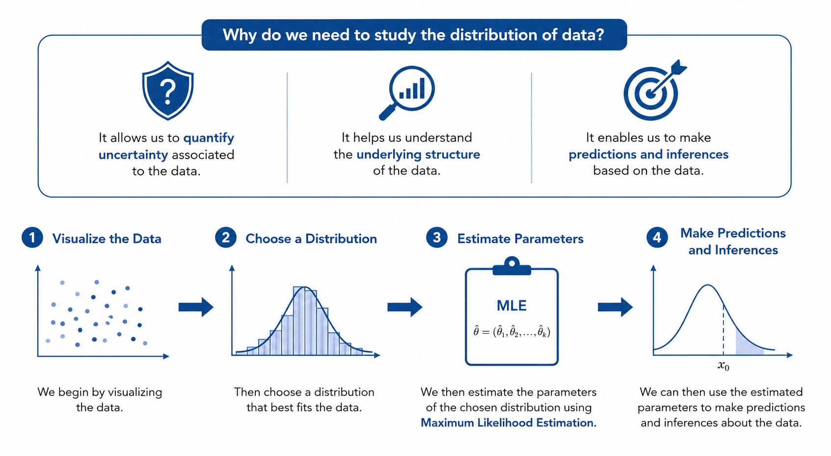
• Using the visualization, we can choose a suitable family of distibution for the data that depends on a parameter \(\color{red}{\theta}\).
• Then, for a fixed set of \(n\) i.i.d. observations \(\{x_1,x_2,...,x_n\}\) drawn from this population, the likelihood function is defined as: \[L(\color{red}{\theta})=f(x_1,x_2,...,x_n|\color{red}{\theta})=\prod_{i=1}^{n} f(x_i|\color{red}{\theta})\geq 0\]

• Maximum Likelihood Estimator \(\color{red}{\widehat{\theta}}\) is the value that maximizes \(L(\color{red}{\theta})\), \[L(\color{red}{\widehat{\theta}})=\max_{\color{red}{\theta}}L(\color{red}{\theta}).\]

Log-likelihood function

• Likelihood function is often difficult to work with as it’s a product of probabilities and can be very small.
• Log-likelihood is an easier objective function to be maximized in order to find MLE: \[\ell(\color{red}{\theta}) = \log L(\color{red}{\theta})= \sum_{i=1}^n \log f(x_i|\color{red}{\theta}).\]

• Maximum Likelihood Estimator \(\color{red}{\widehat{\theta}}\) also maximizes \(\ell(\color{red}{\theta})\), \[\ell(\color{red}{\widehat{\theta}})=\max_{\color{red}{\theta}}\ell(\color{red}{\theta}).\]

Summary

Application: Total Pregnancies

• What’s probability distribution is suitable for Total Pregnancies?
• Model: \(X \sim \mathcal{P}(\color{red}{\lambda})\) for some \(\color{red}{\lambda}>0\).
• Data: Assume \(x_1,...,x_n\) are from the above population and independent.
• Log-likehood: \(\ell(\color{red}{\lambda})=\sum_{k=1}^n[-\color{red}{\lambda}+x_k\log(\color{red}{\lambda})-\log(x_k!)].\)

• Optimization: \[\frac{d\ell(\color{red}{\lambda})}{d\color{red}{\lambda}}=\sum_{k=1}^n\left(-1+\frac{x_k}{\color{red}{\lambda}}\right).\]
• MLE \(\color{red}{\widehat{\lambda}}\) makes \(\frac{d\ell(\color{red}{\widehat{\lambda}})}{d\color{red}{\lambda}}=0\). \[\begin{align*}\Leftrightarrow \sum_{k=1}^n(-1+\frac{x_k}{\color{red}{\widehat{\color{red}{\lambda}}}})&=0\\ \Leftrightarrow\color{red}{\widehat{\lambda}}&=\frac{1}{n}\sum_{k=1}^nx_k.\end{align*}\]
• MLE \(\color{red}{\widehat{\lambda}}=\overline{X}_n=\) 2.38.

Data vs Theoretical Distribution

Data

Simulation

• The choice of your model matters!
• How about trying \(X\sim\mathcal{E}(\color{red}{\lambda})\)?

4 Simulation Methods

4.1 Uniform Random Variable

Linear Congruential Generator (LCG)

• Fact We humans cannot product real randomness!
• Random numbers producted by computer are called pseudorandom numbers.
• LCG is a method to generate pseudorandom uniform numbers by generating a sequence of large integers and then mapping them to the interval \([0,1]\).
• Park-Miller LCG (1988) chose \(a=7^5\), \(b=0\), and \(m=2^{31}-1\):
  • Set seed \(X_0\in\{0,1,...,m-1\}\), then generate \(u_{n+1}=\frac{X_{n+1}}{m}\),
  • \(X_{n+1} = (a \cdot X_n + b) \mod m\).

4.2 Other Distributions

Bernoulli Distribution

• Standard Uniform Distribution allows us to generate almost every other common distributions.
• Bernoulli Distribution can be generated very easily from a uniform distribution.
• Let \(p\) be the probability of success, then:
  • Generate a random number \(u\sim{U}[0,1]\),
  • If \(u<p\), return \(X=1\) (success),
  • Otherwise, return \(X=0\) (failure).
• Check that \(X\sim\mathcal{B}(p)\).

Binomial Distribution

• From Bernoulli Distribution, we can generate a Binomial Distribution by summing up \(n\) independent Bernoulli trials:
  • Initialization: \(n,p\)
  • We generate \(n\) trails of \(X_i\sim\mathcal{B}(p)\), let \(Y=\sum_{i=1}^{n} X_i\)
• Check that \(Y\sim\mathcal{B}(n,p)\).

Number of eggs (n)

Hatching probability (p)

Number of chicks: 0

Exponential Distribution

• From Uniform Distribution, we can generate an Exponential Distribution using Inverse Method.
• Definition: Cummulative Distribution Function (CDF) of a random variable \(X\) is a function \(F(x)=\mathbb{P}(X\leq x)\).
  • If \(X\) is discrete, \(F(x)=\sum_{x_i\leq x} \mathbb{P}(X=x_i)\), the sum of PMF.
  • If \(X\) is continuous, \(F(x)=\int_{-\infty}^{x}f(x)dx\), where \(f\) is its PDF.
• Inverse Transform Sampling: if \(X\) is a RV with CDF \(F(x)\), and \(U\sim U(0,1)\), then \(Y=F^{-1}(U)\) has the same distribution as \(X\).
• Apply to Exponential Distribution
  • Simulate \(U\sim U(0,1)\),
  • Compute \(X=-\frac{1}{\lambda}\log(1-U)\), then \(X\sim {\cal E}(\color{red}{\lambda})\).

Poisson Distribution

• From Exponential Distribution of parameter \(\color{red}{\lambda}\), we can generate a Poisson RV with parameter \(\lambda\) by counting the number of events occur before the total times is \(1\).
• Simulatioin:
  • Simulate \(X_1,X_2,..\sim{\cal E}(\color{red}{\lambda})\),
  • Let \(S_n=X_1+X_2+\cdots+X_n\),
  • Let \(N=\max\{n| S_n\leq 1\}\), then \(N\sim {\cal P}(\color{red}{\lambda})\).

import numpy as np
def poisson_from_exponential(lam):
    t = 0
    n = 0
    while True:
        t += np.random.exponential(1 / lam)
        if t > 1:
            return n
        n += 1

More details can be found here: Supplementary Notes on Simulation Methods.

🥳 Yeahhhh 🥂!!!

Let’s take a break!

Party time 🎉🎉🎉

• Link: https://forms.cloud.microsoft/r/re1ZtCwmMK