import numpy as np
import matplotlib.pyplot as plt
from scipy import stats
from sklearn.tree import DecisionTreeRegressorLab 5: Bootstrap Methods
Course: INS-605: Data Analysis II
Lecturer: Sothea HAS, PhD
- Student name: …
- ID: …
The jupyter notebook can be downloaded here.
0. Before You Start
In the lecture, you saw that Bootstrapping lets us approximate the sampling distribution of an estimator \(\widehat\theta\) by repeatedly resampling with replacement from the single dataset we have, instead of collecting new data.
TipBootstrap procedure (recap)
- Initialize \(B\) (number of bootstrap samples, typically \(\ge 1000\)) and the data \(D=\{x_1,\dots,x_n\}\).
- For \(b=1,\dots,B\):
- Draw \(D_b^*\) by sampling with replacement from \(D\) (same size \(n\)).
- Compute \(\widehat\theta_b\), the statistic of interest, on \(D_b^*\).
- Collect \(\widehat\Theta = [\widehat\theta_1,\dots,\widehat\theta_B]\) — this approximates the sampling distribution of \(\widehat\theta\).
Today, you will use \(\widehat\Theta\) to build four different types of bootstrap confidence intervals for a statistic, compare them to each other (and to a classical analytic CI), and then take a first look at how bootstrap ideas power Bagging in Machine Learning.
Roadmap
| Section | What you’ll do |
|---|---|
| 1. Warm-up | Simulate data, build a generic bootstrap resampler, look at a sampling distribution |
| 2. Four CIs | Implement the Percentile, Basic (reflection), Normal-approximation CIs, and Bias-corrected CI |
| 3. Compare | Put all CIs side-by-side, compare to a classical CI, try a statistic with no closed form |
| 4. Bootstrap in ML | A first taste of Bagging: does averaging bootstrap-trained models reduce variance? |
| 5. Going further (take home, ~30-45 min) | Coverage simulation, a bootstrap CI for a correlation, and B vs. bagging variance |
Sections 1-4 are designed for our 75-minute session; Section 5 is for you to finish at home.
Run the cell below to load the packages we need.
1. Warm-up: Simulating Data & the Bootstrap Sampling Distribution
1.1. A Small, Skewed Sample
Imagine we tracked the session duration (in minutes) of \(n=25\) visitors on a website. Session durations are typically right-skewed: most visits are short, a few are very long. Run the cell below to simulate such a sample (treat it as our one and only observed dataset \(D\), exactly as in the lecture).
n = 25
session_times = np.round(np.random.lognormal(mean=1.6, sigma=0.7, size=n), 1)
A.1. Statistics and visualization: Compute statistical summary and visualize the distribution of the data above.
import seaborn as sns
import pandas as pd
df = pd.DataFrame(session_times, columns=['session time'])
print(df.describe())
sns.histplot(
    df,
    x = 'session time',
    kde=True,
    color='#292B71'
)
session time
count 25.000000
mean 7.340000
std 7.076722
min 1.000000
25% 2.800000
50% 4.700000
75% 8.300000
max 29.600000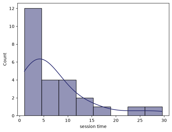
A.2 In a markdown cell, briefly answer: looking at the histogram, would you trust the Normal (Gaussian) approximation of the sampling distribution of the mean here, given the skewness and small \(n=25\)? Why does this matter for building confidence intervals?
A.2. Your answer here:
…
1.2. A Generic Bootstrap Resampler
B. Complete the function below: it should draw B bootstrap samples (each of size n, with replacement) from data, apply stat_func to each, and return the array of B bootstrap estimates. Hint: use np.random.choice().
def bootstrap_estimates(data, stat_func, B=2000):
    """
    Draw B bootstrap samples (with replacement) from `data` and
    return an array of B values of stat_func evaluated on each sample.
    """
    n = len(data)
    estimates = np.zeros(B)
    for b in range(B):
        sample_b = np.random.choice(
            data,
            size=n,
            replace=True)
        estimates[b] = stat_func(sample_b)
    return estimates
C. Use your function to draw \(B=2000\) bootstrap estimates of the mean session duration. Plot a histogram of the bootstrap sampling distribution \(\widehat\Theta\), and report the bootstrap standard error \(\text{SE}(\widehat\theta) = \text{sd}(\widehat\Theta)\).
B = 2000
theta_hat = session_times.mean()  # the original point estimate, from D itself

theta_boot_mean = bootstrap_estimates(session_times, np.mean)
se_boot = theta_boot_mean.std(ddof=1)
2. Constructing Four Types of Bootstrap Confidence Intervals
From lecture, once we have \(\widehat\Theta=[\widehat\theta_1,\dots,\widehat\theta_B]\), there are several ways to turn it into a \((1-\alpha)\) confidence interval for \(\theta\). We’ll implement four of them, using the original point estimate \(\widehat\theta\) (from \(D\) itself) and the bootstrap distribution \(\widehat\Theta\).
TipFour CI recipes
Let \(\widehat\theta_{(q)}\) denote the \(q\)-th percentile of \(\widehat\Theta\), and \(\text{SE}=\text{sd}(\widehat\Theta)\). Let \(\alpha\in(0,1)\) be the error tolerance, therefore \((1-\alpha)\) be the confidence level, one has:
Percentile CI: just use the empirical quantiles of \(\widehat\Theta\) directly: \[\text{CI}_{\text{perc}} = \left[\widehat\theta_{(\alpha/2)},\ \widehat\theta_{(1-\alpha/2)}\right]\]
Basic (reflection) CI: reflect the bootstrap quantiles around the original estimate \(\widehat\theta\) — this corrects for any skewness/bias between \(\widehat\theta\) and the center of \(\widehat\Theta\): \[\text{CI}_{\text{basic}} = \left[2\widehat\theta-\widehat\theta_{(1-\alpha/2)},\ 2\widehat\theta-\widehat\theta_{(\alpha/2)}\right]\]
Normal-approximation CI: assume \(\widehat\Theta\) is approximately Normal and just use its standard deviation with a \(z\)-quantile \(q_{1-\alpha/2}=\Phi^{-1}(1-\alpha/2)\): \[\text{CI}_{\text{norm}} = \left[\widehat\theta - q_{1-\alpha/2}\cdot\text{SE},\ \widehat\theta + q_{1-\alpha/2}\cdot\text{SE}\right]\]
Three of the four use the same \(\widehat\Theta\) — they just summarize it differently. When \(\widehat\Theta\) is symmetric and unbiased, all three should roughly agree.
TipBias-corrected CI
Let \(\widehat\theta_{(q)}\) denote the \(q\)-th percentile of \(\widehat\Theta\), and \(\text{SE}=\text{sd}(\widehat\Theta)\), the Bias-Corrected CI at confidence level \(1-\alpha\) is defined by,
- Bias: \(\displaystyle\text{Bias}_0 = \frac{\#\{b:\widehat\theta_{b}\text{ such that }\widehat\theta_{b}\leq \widehat{\theta}\}}{B}\) the proportion of smaller estimators than the mean.
- Correction: \(\displaystyle c_0=\phi^{-1}(\text{bias}_0)\).
- Redefine the lower and upper boundary: lower boundary \(\alpha_L=\phi(2c_0-q_{1-\alpha/2})\) and upper boundary \(\alpha_U=\phi(2c_0+q_{1-\alpha/2})\).
- Bias-corrected CI: \[\text{CI}_{\text{bias-corrected}}= \left[\widehat{\theta}_{(\alpha_L)},\widehat{\theta}_{(\alpha_U)}\right].\]
2.1. Percentile CI
A. Complete percentile_ci below.
def percentile_ci(theta_boot, alpha=0.05):
    lower = None  # TODO
    upper = None  # TODO
    return lower, upper

ci_perc = percentile_ci(theta_boot_mean)
print(f"Percentile 95% CI: [{ci_perc[0]:.3f}, {ci_perc[1]:.3f}]")
2.2. Basic (Reflection) CI
B. Complete basic_ci below. Notice how it uses theta_hat (from the original data) explicitly, not just \(\widehat\Theta\).
def basic_ci(theta_boot, theta_hat, alpha=0.05):
    lower_perc, upper_perc = percentile_ci(theta_boot, alpha)
    lower = None  # TODO
    upper = None  # TODO
    return lower, upper

ci_basic = basic_ci(theta_boot_mean, theta_hat)
print(f"Basic 95% CI:      [{ci_basic[0]:.3f}, {ci_basic[1]:.3f}]")
2.3. Normal-Approximation CI
C. Complete normal_ci below. Use stats.norm.ppf for the quantile \(q_{1-\alpha/2}\).
def normal_ci(theta_hat, se, alpha=0.05):
    z = None  # TODO: stats.norm.ppf(1 - alpha/2)
    lower = None  # TODO
    upper = None  # TODO
    return lower, upper

ci_norm = normal_ci(theta_hat, se_boot)
print(f"Normal-approx 95% CI: [{ci_norm[0]:.3f}, {ci_norm[1]:.3f}]")
2.4 Bias-corrected CI
D. Complete bias_corrected_CI below.
def bias_corrected_ci(theta_hat, alpha=0.05):
    bias = None # TODO: compute bias
    c0 = None # TODO: Compute correction c0
    q = None  # TODO: stats.norm.ppf(1 - alpha/2)
    aL = None # TODO: compute lower bound of percentage
    aU = None # TODO: compute upper bound of percentage
    lower = None  # TODO
    upper = None  # TODO
    return lower, upper

ci_bias_corrected = bias_corrected_ci(theta_hat)
print(f"Normal-approx 95% CI: [{ci_bias_corrected[0]:.3f}, {ci_bias_corrected[1]:.3f}]")
3. Comparing the Confidence Intervals
3.1. A Classical Baseline: the \(t\)-interval
For the mean specifically, classical (non-bootstrap) statistics gives us the analytic \(t\)-interval: \[\text{CI}_t = \left[\bar x - t_{1-\alpha/2,\,n-1}\cdot\frac{s}{\sqrt n},\ \bar x + t_{1-\alpha/2,\,n-1}\cdot\frac{s}{\sqrt n}\right]\]
A. Compute this interval using stats.t.interval with \(s=\) sample std (ddof=1).
alpha = 0.05
s = None # TODO: Compute std of the session_times data.
se_analytic = None # Compute SE by s / np.sqrt(n)

ci_t = None  # TODO: use the formula above.
print(f"Classical t-interval: [{ci_t[0]:.3f}, {ci_t[1]:.3f}]")
3.2. Side-by-Side Comparison
B. Complete the plotting code below to visualize all four 95% CIs for the mean session duration on the same axis (as horizontal error bars), together with \(\widehat\theta\).
ci_dict = {
    'Percentile': ci_perc,
    'Basic': ci_basic,
    'Normal-approx': ci_norm,
    'Bias-correction': ci_bias_corrected,
    'Classical t': ci_t,
}

fig, ax = plt.subplots(figsize=(7, 4))
for i, (name, (lo, hi)) in enumerate(ci_dict.items()):
    center = None  # TODO: midpoint of (lo, hi)
    half_width = None  # TODO: half of (hi - lo)
    ax.errorbar(center, i, xerr=half_width, fmt='o', capsize=5, color='#345a8b')
ax.axvline(theta_hat, color='gray', linestyle='--', label=r'$\hat\theta$')
ax.set_yticks(range(len(ci_dict))); ax.set_yticklabels(ci_dict.keys())
ax.set_xlabel('Mean session duration (minutes)'); ax.set_title('95% CIs for the mean: four methods')
ax.legend(); plt.tight_layout(); plt.show()
C. In a markdown cell, briefly answer:
Which interval is widest? Narrowest? Does that surprise you given \(n=25\) and the skewness you saw in Section 1?
The Basic and Percentile CIs are both built from the same \(\widehat\Theta\) — why can they still give different bounds?
C. Your answer here:
…
…
3.3. Where Bootstrap Really Shines: A Statistic With No Simple Formula
The \(t\)-interval above only works because we have a textbook formula for the standard error of the mean. Bootstrap doesn’t need one — it works for (almost) any statistic. Let’s try the median, for which there is no simple closed-form CI.
D. Repeat the bootstrap + four-CI pipeline for np.median instead of np.mean (reuse your functions!). Print all four CIs.
theta_hat_med = np.median(session_times)
theta_boot_med = None  # TODO: compute median instead.
se_boot_med = None  # TODO

ci_perc_med = None  # TODO
ci_basic_med = None  # TODO
ci_norm_med = None  # TODO

print(f"Median (theta_hat):   {theta_hat_med:.3f}")
print(f"Percentile 95% CI:    [{ci_perc_med[0]:.3f}, {ci_perc_med[1]:.3f}]")
print(f"Basic 95% CI:         [{ci_basic_med[0]:.3f}, {ci_basic_med[1]:.3f}]")
print(f"Normal-approx 95% CI: [{ci_norm_med[0]:.3f}, {ci_norm_med[1]:.3f}]")
E. In one or two sentences: why is there no simple \(t\)-interval equivalent for the median, and why does that make bootstrap especially valuable here?
E. Your answer here:
…
4. Bootstrap in Machine Learning: A First Taste of Bagging
Recall from lecture: Bagging (Bootstrap Aggregating) trains one model \(f_b\) per bootstrap sample \(D_b^*\), then averages: \(\widehat f_{\text{bag}}(x)=\frac1B\sum_b f_b(x)\). A single model trained on one dataset can be unstable (high variance); averaging over many bootstrap-trained models tends to stabilize the prediction.
Let’s see this with a small regression example.
np.random.seed(605)
n_pts = 30
x_train = np.sort(np.random.uniform(0, 10, n_pts))          # For training
y_train = np.sin(x_train) + np.random.normal(0, 0.3, n_pts) # For training
x_grid = np.linspace(0, 10, 200).reshape(-1, 1)             # For testing

plt.scatter(x_train, y_train, color='#345a8b', label='Training data')
plt.plot(x_grid, np.sin(x_grid), color='black', linestyle='--', label='True function sin(x)')
plt.legend(); plt.title('A small, noisy regression dataset'); plt.show()
A. Train one DecisionTreeRegressor (max_depth=4) on the full training set, and plot its prediction curve over x_grid against the true function. Decision trees trained on few data points tend to be quite unstable/wiggly — keep this in mind for the next part.
tree_single = DecisionTreeRegressor(max_depth=4, random_state=605)
tree_single.fit(None, None)  # TODO: fit on x_train (reshaped to a column) and y_train
y_single = None  # TODO: predict on x_grid

plt.scatter(x_train, y_train, color='#345a8b', alpha=0.5)
plt.plot(x_grid, np.sin(x_grid), color='black', linestyle='--', label='True function')
plt.plot(x_grid, y_single, color='#d97f2e', label='Single tree')
plt.legend(); plt.title('A single decision tree'); plt.show()
B. Now build a small Bagging ensemble: train \(B=100\) trees, each on an independent bootstrap sample of (x_train, y_train) (sample the indices with replacement, size \(n\)), then average their predictions on x_grid. Plot the ensemble average against the single tree and the truth.
B_bag = 100
predictions = np.zeros((B_bag, len(x_grid)))

for b in range(B_bag):
    idx = None  # TODO: sample indices with replacement to generate bootstrap sample
    x_b, y_b = x_train[idx], y_train[idx]   # select those bootstrap sample from the data
    tree_b = None # TODO: build the tree on the bootstrap samples
    tree_b.fit(None, None) # Fit the model on the bootstrap data
    predictions[b] = None  # TODO: predict it on x_grid

y_bagged = None  # TODO: average predictions over the B_bag trees (axis=0)

plt.scatter(x_train, y_train, color='#345a8b', alpha=0.4)
plt.plot(x_grid, np.sin(x_grid), color='black', linestyle='--', label='True function')
plt.plot(x_grid, y_single, color='#d97f2e', label='Single tree')
plt.plot(x_grid, y_bagged, color='#2e8b57', linewidth=2, label=f'Bagged ({B_bag} trees)')
plt.legend(); plt.title('Single tree vs. Bagging'); plt.show()
C. Compute the pointwise variance across the \(B=100\) bootstrap-trained trees at each grid point (predictions.var(axis=0)), and report its average. Then, in a markdown cell, connect what you see to the lecture’s variance formula \(\mathbb V(\bar f)=\sigma^2\left[\rho+\frac{1-\rho}{B}\right]\) — does averaging make the prediction perfectly stable, or is there a limit?
pointwise_var = None  # TODO: compute variance of the prediction using 'predictions' above.
print(f"Average pointwise variance across the ensemble: {pointwise_var.mean():.4f}")
D. Your answer here:
…
5. Going Further (Homework)
The sections below are for you to complete after class, at your own pace. They dig a bit deeper into ideas we only touched on today.
5.1. Does a 95% CI Really Cover 95% of the Time?
A 95% CI means: if we repeated the whole sampling + CI-construction process many times, about 95% of the resulting intervals would contain the true parameter. Since we simulated session_times from a known lognormal distribution, we actually know the true population mean, and we can check this directly!
A. The true mean of a \(\text{Lognormal}(\mu,\sigma)\) is \(\mathbb E[X]=e^{\mu+\sigma^2/2}\). Compute it for \(\mu=1.6,\ \sigma=0.7\) (matching Section 1.1).
B. Write a loop that, for n_repeats = 200 times:
draws a fresh sample of size \(n=25\) from the same lognormal distribution,
builds the Percentile, Basic, and Normal-approx 95% CIs for the mean (using \(B=500\) bootstrap replicates to keep things fast), and
records whether each CI contains the true mean. Report the empirical coverage (fraction of intervals containing the true mean) for each method. (This will take a little while to run — that’s fine, let it finish while you read ahead.)
true_mu, true_sigma = 1.6, 0.7
true_mean = None  # TODO: apply formula of expectation in question A. above in here.
print(f"True population mean: {true_mean:.4f}")

n_repeats = 200
B_small = 500
covered = {'Percentile': 0, 'Basic': 0, 'Normal-approx': 0}

for r in range(n_repeats):
    sample_r = None  # TODO: draw a fresh lognormal sample, size n, params (true_mu, true_sigma)
    theta_hat_r = sample_r.mean()
    theta_boot_r = bootstrap_estimates(sample_r, np.mean, B_small)
    se_r = theta_boot_r.std(ddof=1)

    lo_p, hi_p = percentile_ci(theta_boot_r)
    lo_b, hi_b = basic_ci(theta_boot_r, theta_hat_r)
    lo_n, hi_n = normal_ci(theta_hat_r, se_r)

    covered['Percentile']    += (lo_p <= true_mean <= hi_p)
    covered['Basic']         += (lo_b <= true_mean <= hi_b)
    covered['Normal-approx'] += (lo_n <= true_mean <= hi_n)

for method, count in covered.items():
    print(f"{method:15s}: empirical coverage = {count/n_repeats:.3f}")
C. Is the empirical coverage close to the nominal 95%? If one method’s coverage is noticeably off, which one is it, and can you connect that back to what you observed about skewness in Section 1?
C. Your answer here:
…
5.2. Bootstrap CI for a Correlation Coefficient
Bootstrap is especially handy for statistics like the Pearson correlation \(r\), which has an awkward sampling distribution (bounded in \([-1,1]\), skewed when \(|r|\) is large) — an exact analytic CI exists (Fisher’s \(z\)-transform) but is easy to get wrong, whereas the bootstrap recipe is exactly the same as before.
A. Run the cell below to simulate \(n=40\) paired observations \((u_i, v_i)\) with true correlation around 0.6.
np.random.seed(47)
n_corr = 40
mean_uv = [0, 0]
cov_uv = [[1, 0.6], [0.6, 1]]
uv = np.random.multivariate_normal(mean_uv, cov_uv, size=n_corr)
u, v = uv[:, 0], uv[:, 1]

plt.scatter(u, v, color='#345a8b'); plt.xlabel('u'); plt.ylabel('v')
plt.title(f'Sample correlation r = {np.corrcoef(u, v)[0,1]:.3f}'); plt.show()
B. Since our bootstrap_estimates function expects a single 1-D data array, resample row indices of the paired data instead (with replacement), and compute the correlation on each resampled pair. Complete the function bootstrap_correlation below, then build the Percentile 95% CI for the true correlation.
def bootstrap_correlation(u, v, B=2000):
    n_uv = len(u)
    r_boot = np.zeros(B)
    for b in range(B):
        idx = None  # TODO: np.random.choice(n_uv, size=n_uv, replace=True)
        r_boot[b] = None  # TODO: np.corrcoef(u[idx], v[idx])[0, 1]
    return r_boot

r_hat = np.corrcoef(u, v)[0, 1]
r_boot = None  # TODO: apply the function above on u, v and B=2000
ci_perc_r = None  # TODO: compute the percentile on r_boot

print(f"Sample correlation r:  {r_hat:.3f}")
print(f"Percentile 95% CI:     [{ci_perc_r[0]:.3f}, {ci_perc_r[1]:.3f}]")
5.3. Bonus: How Does \(B\) Affect Bagging’s Variance Floor?
Recall from lecture: with pairwise model correlation \(\rho\), \(\mathbb V(\bar f)=\sigma^2\left[\rho+\frac{1-\rho}{B}\right]\to\rho\sigma^2\) as \(B\to\infty\) — more trees help, but only up to a point.
A. Using the same setup as Section 4, repeat the bagging experiment for a few different ensemble sizes, e.g. B_values = [1, 5, 20, 50, 100, 300]. For each \(B\), train the ensemble (you can reuse your loop from Section 4.2) and record the average pointwise variance across grid points. Plot average variance vs. \(B\). Does it plateau, as the formula predicts?
B_values = [1, 5, 20, 50, 100, 300, 500]
avg_variances = []

for B_val in B_values:
    preds = np.zeros((B_val, len(x_grid)))
    for b in range(B_val):
        idx = None # generate random indices for bootstrap sample
        x_b, y_b = None, None # # draw bootstrap sample
        tree_b = DecisionTreeRegressor(max_depth=4, random_state=b)
        tree_b.fit(None, None) # fit. model on the bootstrap sample
        preds[b] = None # Prediction
    avg_variances.append(None)  # TODO: average pointwise variance for this B_val

plt.plot(B_values, avg_variances, marker='o', color='#345a8b')
plt.xlabel('Number of bootstrap trees B'); plt.ylabel('Average pointwise variance')
plt.title('Does more trees keep reducing variance forever?'); plt.show()
Wrap-up
In this lab you:
- Built a generic bootstrap resampler and used it to approximate the sampling distribution of the mean (Section 1).
- Implemented and compared four types of bootstrap CIs — Percentile, Basic (reflection), and Normal-approximation — against a classical \(t\)-interval (Sections 2-3).
- Saw bootstrap’s real advantage: it works just as easily for statistics with no simple formula, like the median (Section 3.3).
- Connected bootstrap resampling to Bagging in Machine Learning, and saw how averaging bootstrap-trained models reduces prediction variance (Section 4).
- (At home) Verified empirical coverage of your CIs, built a bootstrap CI for a correlation coefficient, and explored how the bagging variance floor depends on \(B\) (Section 5).
The core idea carries through every section: treat your one dataset as a stand-in for the population, resample it many times, and let the resulting variation tell you how much to trust your estimate.